Alouette Reservoir Kokanee Population Analysis 2015
The suggested citation for this analytic report is:
Thorley, J.L., Hogan, P.M., Irvine, R.L. and Campos, M. (2016) Alouette Reservoir Kokanee Population Analysis 2015. A Poisson Consulting Analysis Report. URL: https://www.poissonconsulting.ca/f/1819975990.
Background
The Kokanee Age Structure Population Analysis (ALUMON #6) is a multi-year study to address potential impacts of reservoir operations on the reservoirs’ kokanee (Oncorhynchus nerka) population (Andrusak 2014). As part of the Alouette Reservoir Water Use Plan (WUP), the study’s focus is to address whether the current kokanee population is recruitment limited and if any identified recruitment limitation is related to BC Hydro operations.
The management questions outlined in the WUP terms of reference were as follows:
- The size-at-age of the kokanee population remains stable, or decreases with time once the standing crop has stabilized with the annual addition of fertilizer.
- Drops in fry abundance, relative to estimates in previous years and to that predicted by estimates of mature kokanee, are uncorrelated with the extent of the reservoir fluctuations during the spawning and incubation period.
- Whether drops in fry abundance persist through time and cause an impact on the abundance of mature kokanee.
Methods
Data Preparation
The hydroacoustic and gillnetting data from 1998-2014 on the Alouette Reservoir were provided by Redfish Consulting Ltd.(G. Andrusak) and BC MNFLRO (S. Harris).
Size-at-Age
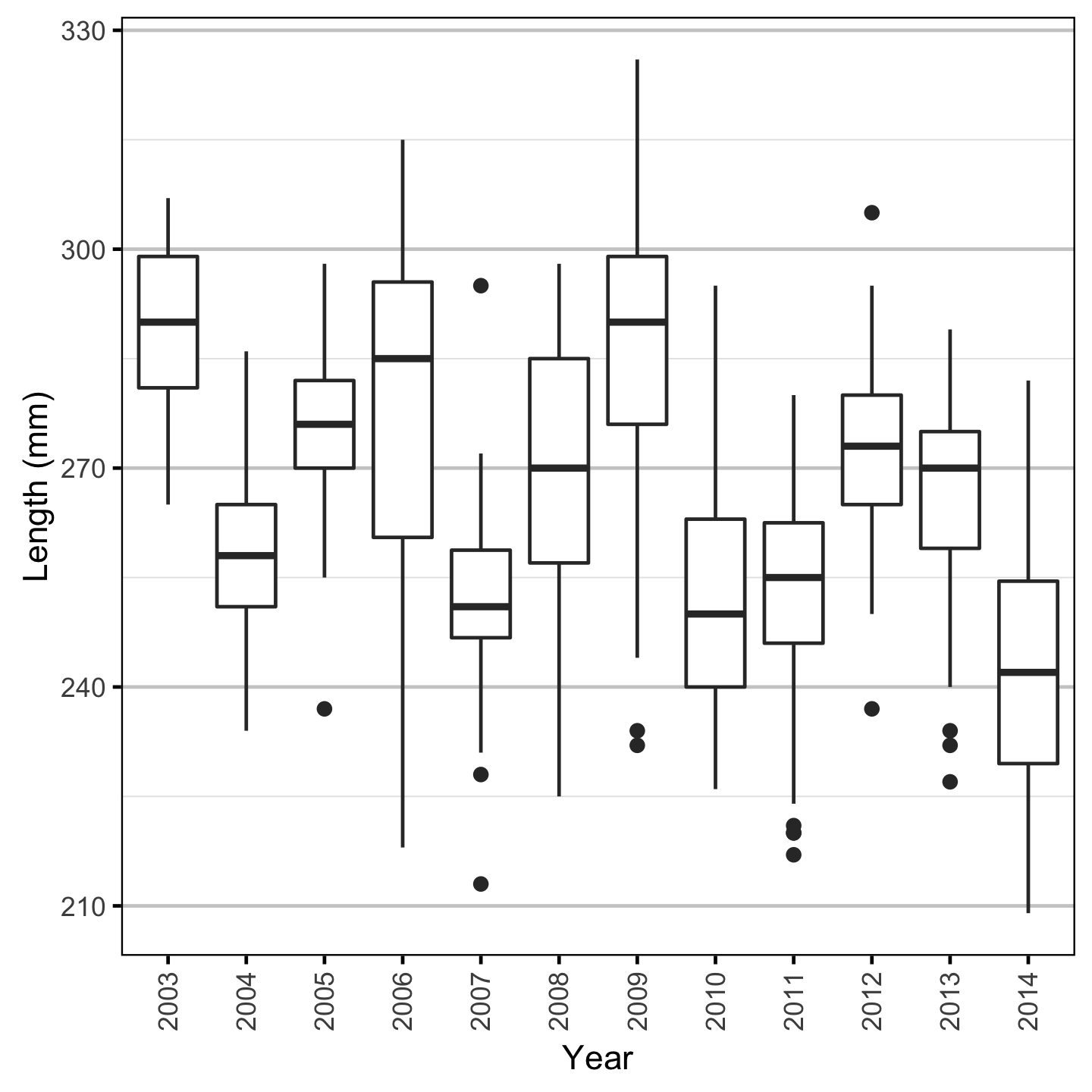
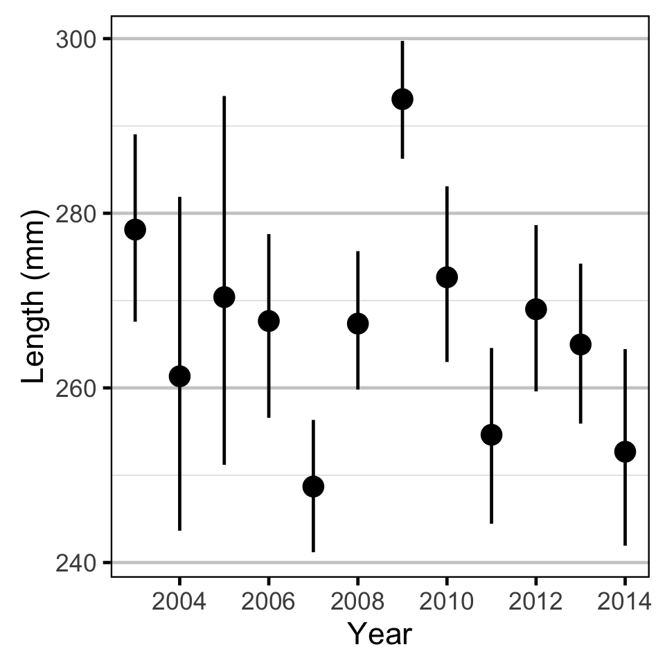
The data used for size-at-age analysis were Kokanee Age-3 lengths obtained through gillnetting surveys from 2003-2014.
During the size-at-age survey data preparation:
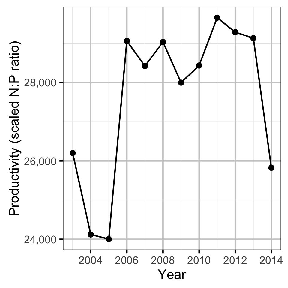
- The productivity was calculated as the N:P ratio from 2008-2013 of 7.45 multiplied by the nutrient with the lower value in the ratio (P).
- Standing crop was considered to be stabilized in 2003.
- Fish that were netted in July were removed.
Stock-Recruitment
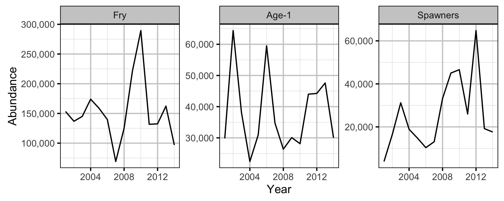
The data used for stock-recruitment analysis were obtained through hydroacoustic surveys completed in water depths 10m or greater from years 2001-2014. Spawners were defined as fish that were classified as Age-2 or Age-3+ and fry were fish classified as Age-0 from the decibel ranges used by MNFLRO. The spawning and incubation period was considered to be October 15 to February 28.
During the size-at-age survey data preparation:
- Fry numbers were multiplied by 0.92 to correct for non-Kokanee detections.
Statistical Analysis
Hierarchical Bayesian models were fitted to the count data using R version 3.2.3 (Team 2013) and JAGS 4.0.1 (Plummer 2015) which interfaced with each other via jaggernaut 2.3.1 (Thorley 2013). For additional information on hierarchical Bayesian modelling in the BUGS language, of which JAGS uses a dialect, the reader is referred to (Kery and Schaub 2011, 41–44).
Unless specified, the models assumed vague (low information) prior distributions (Kery and Schaub 2011, 36). The posterior distributions were estimated from a minimum of 1,000 Markov Chain Monte Carlo (MCMC) samples thinned from the second halves of three chains (Kery and Schaub 2011, 38–40). Model convergence was confirmed by ensuring that Rhat (Kery and Schaub 2011, 40) was less than 1.1 for each of the parameters in the model (Kery and Schaub 2011, 61).
The posterior distributions of the fixed (Kery and Schaub 2011, 75) parameters are summarised in terms of a point estimate (mean), lower and upper 95% credible limits (2.5th and 97.5th percentiles), the standard deviation (SD), percent relative error (half the 95% credible interval as a percent of the point estimate) and significance (Kery and Schaub 2011, 37, 42).
Variable selection was achieved by dropping insignificant (Kery and Schaub 2011, 37, 42) fixed (Kery and Schaub 2011, 77–82) variables and uninformative random variables. A fixed variables was considered to be insignificant if its significance was \(\geq\) 0.05 while a random variable was considered to be uninformative if its percent relative error was \(\geq\) 80%. The Deviance Information Criterion (DIC) was not used because it is of questionable validity when applied to hierarchical models (Kery and Schaub 2011, 469).
The results are displayed graphically by plotting the modelled relationships between particular variables and the response with 95% credible intervals (CRIs) with the remaining variables held constant. In general, continuous and discrete fixed variables are held constant at their mean and first level values respectively while random variables are held constant at their typical values (expected values of the underlying hyperdistributions) (Kery and Schaub 2011, 77–82). Where informative the influence of particular variables is expressed in terms of the effect size (i.e., percent change in the response variable) with 95% CRIs (Bradford, Korman, and Higgins 2005).
Size-at-Age
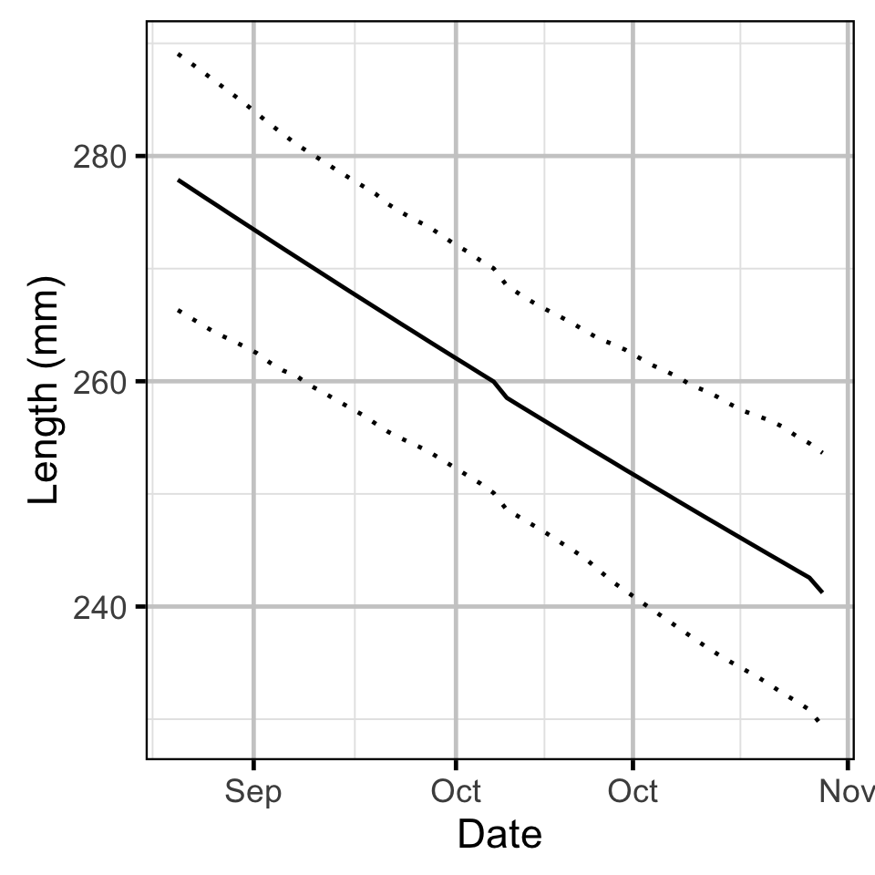
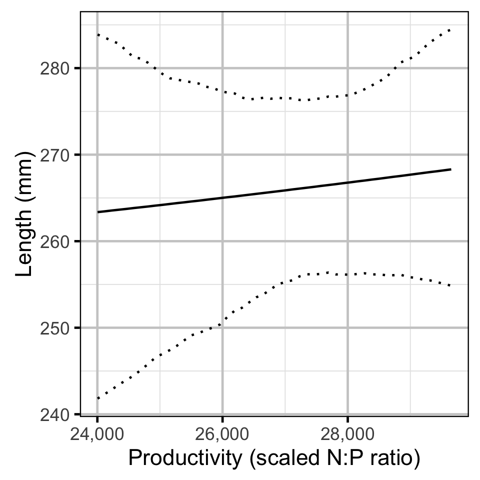
The size-at-age of Age-3 Kokanee was analysed using a hierarchical Bayesian generalized mixed effects model. Key assumptions of this model include:
- Size-at-age varies with productivity and day of the year.
- Size-at-age varies randomly with year and location within year.
- The residual variation in size-at-age is log-normally distributed.
Preliminary analyses indicated that the type of net set and the spawner abundance were not significant predictors of size-at-age.
Stock-Recruitment
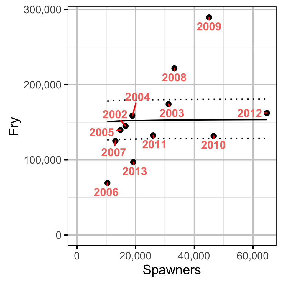
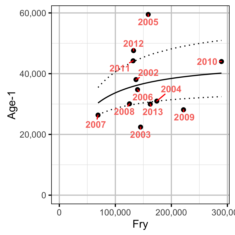
The spawner-to-fry and fry-to-age-1 stock-recruitment relationships were both analysed using a Bayesian Beverton-Holt model.
Key assumptions of this model include:
- Recruitment varies with stock as described by a Beverton-Holt curve.
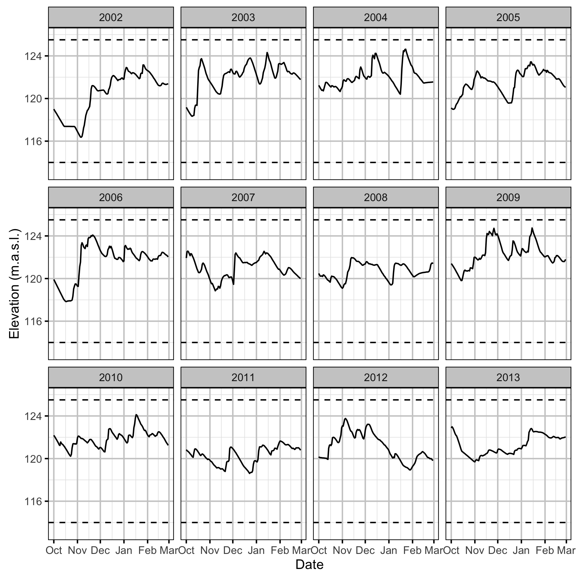
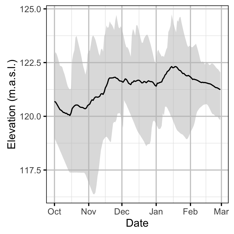
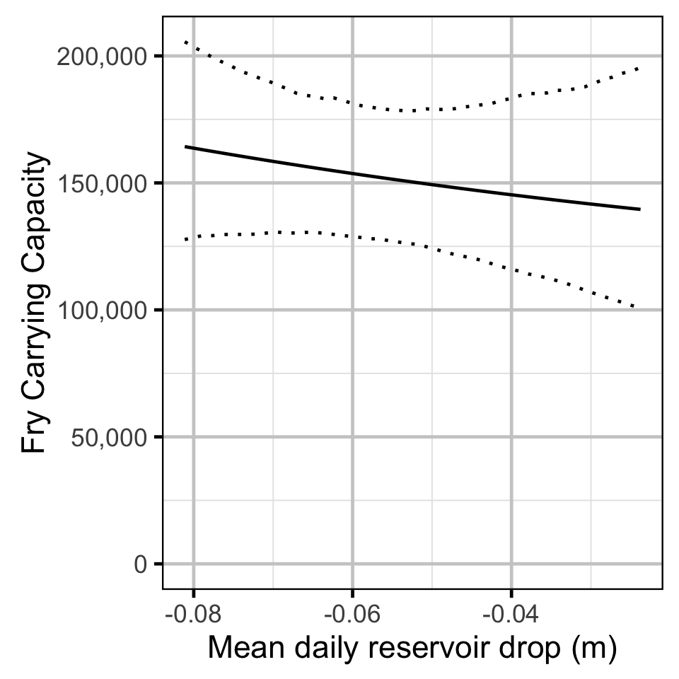
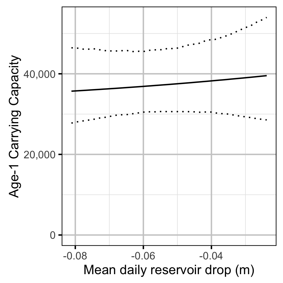
- Recruitment varies with the mean daily drop in reservoir elevation from October 15 to February 28.
- The residual variation in recruitment is log-normally distributed.
Model Code
The JAGS model code, which uses a series of naming conventions, is presented below.
Size-At-Age
| Variable/Parameter | Description |
|---|---|
bLength |
Intercept for log(eLength) |
bLengthDayte |
Effect of Dayte on log(eLength) |
bLengthLocationYear[i, j] |
Effect of ith Location in jth Year on log(eLength) |
bLengthProductivity |
Effect of Productivity on log(eLength) |
bLengthYear[i] |
Effect of ith Year on log(eLength) |
Dayte[i] |
Day of the year of capture of ith fish |
eLength[i] |
Predicted length of ith fish |
Length[i] |
Measured length of ith fish |
Location[i] |
Location of capture of ith fish |
Productivity[i] |
Productivity in year of capture of ith fish |
sLength |
Standard deviation of residual variation in log(eLength) |
sLengthLocationYear |
Standard deviation of effect of ith Location in jth Year on log(eLength) |
sLengthYear |
Standard deviation of effect of ith Year on log(eLength) |
Year[i] |
Year of capture of ith fish |
Size-At-Age - Model1
model{
  bLength ~ dnorm(5, 5^-2)

  bLengthDayte ~ dnorm(0, 5^-2)

  bLengthProductivity ~ dnorm(0, 5^-2)

  sLengthYear ~ dunif(0, 5)
  for (i in 1:nYear) {
      bLengthYear[i] ~ dnorm(0, sLengthYear^-2)
  }

  sLengthLocationYear ~ dunif(0, 5)
  for (i in 1:nLocation) {
    for(j in 1:nYear) {
      bLengthLocationYear[i, j] ~ dnorm(0, sLengthLocationYear^-2)
    }
  }

  sLength ~ dunif(0, 5)

  for(i in 1:length(Length)){
    log(eLength[i]) <- bLength
                     + bLengthDayte * Dayte[i]
                     + bLengthProductivity * Productivity[i]
                     + bLengthYear[Year[i]]
                     + bLengthLocationYear[Location[i], Year[i]]

    Length[i] ~ dlnorm(log(eLength[i]), sLength^-2)
  }
}
Spawners To Fry
| Variable/Parameter | Description |
|---|---|
bElevationalDrop |
Effect of ElevationalDrop on log(eRecruits) |
ElevationalDrop[i] |
Mean daily drop in reservoir elevation in ith spawn year |
eRecruits[i] |
Expected number of recruits in ith spawn year |
K |
Carrying capacity of the environment |
R0 |
Proliferation rate per generation |
Recruits[i] |
Observed number of recruits in ith spawn year |
sRecruits |
Standard deviation of residual variation in log(eRecruits) |
Stock[i] |
Observed number of spawners in ith spawn year |
Spawners To Fry - Model1
model {
  K ~ dnorm(10^3, (10^3 /2)^-2) T(1, )
  R0 ~  dnorm(10^5, (10^5)^-2) T(10^4, 10^7)

  bElevationalDrop ~ dnorm(0, 5^-2)

  sRecruits ~ dunif(0, 5)

  for(i in 1:length(Stock)){
    log(eRecruits[i]) <- log(K * Stock[i] / (1 + Stock[i] * (K - 1) / R0))
                       + bElevationalDrop * ElevationalDrop[i]

    Recruits[i] ~ dlnorm(log(eRecruits[i]), sRecruits^-2)
  }
}
Fry To Age-1
| Variable/Parameter | Description |
|---|---|
bElevationalDrop |
Effect of ElevationalDrop on log(eRecruits) |
ElevationalDrop[i] |
Mean daily drop in reservoir elevation in ith spawn year |
eRecruits[i] |
Expected number of recruits in ith spawn year |
K |
Carrying capacity of the environment |
R0 |
Proliferation rate per generation |
Recruits[i] |
Observed number of recruits in ith spawn year |
sRecruits |
Standard deviation of residual variation in log(eRecruits) |
Stock[i] |
Observed number of spawners in ith spawn year |
Fry To Age-1 - Model1
model {
  K ~ dnorm(2, 1^-2) T(1, )
  R0 ~  dnorm(10^4, (10^3)^-2) T(0, )

  bElevationalDrop ~ dnorm(0, 5^-2)

  sRecruits ~ dunif(0, 5)

  for(i in 1:length(Stock)){
    log(eRecruits[i]) <- log(K * Stock[i] / (1 + Stock[i] * (K - 1) / R0))
                       + bElevationalDrop * ElevationalDrop[i]

    Recruits[i] ~ dlnorm(log(eRecruits[i]), sRecruits^-2)
  }
}
Results
Model Parameters
The posterior distributions for the fixed (Kery and Schaub 2011 p. 75) parameters in each model are summarised below.
Size-At-Age
| Parameter | Estimate | Lower | Upper | SD | Error | Significance |
|---|---|---|---|---|---|---|
| bLength | 5.5853800 | 5.5461800 | 5.622780 | 0.0184600 | 1 | 0.0010 |
| bLengthDayte | -0.0027770 | -0.0036510 | -0.001861 | 0.0004620 | 32 | 0.0010 |
| bLengthProductivity | 0.0000034 | -0.0000154 | 0.000023 | 0.0000096 | 570 | 0.7066 |
| sLength | 0.0530720 | 0.0500760 | 0.056145 | 0.0015270 | 6 | 0.0010 |
| sLengthLocationYear | 0.0194600 | 0.0102700 | 0.029700 | 0.0049600 | 50 | 0.0010 |
| sLengthYear | 0.0573900 | 0.0337000 | 0.101740 | 0.0168000 | 59 | 0.0010 |
| Convergence | Iterations |
|---|---|
| 1.01 | 50000 |
Spawners To Fry
| Parameter | Estimate | Lower | Upper | SD | Error | Significance |
|---|---|---|---|---|---|---|
| bElevationalDrop | -2.9600 | -10.9100 | 5.4800e+00 | 4.150e+00 | 280 | 0.4492 |
| K | 1009.0000 | 154.0000 | 1.9330e+03 | 4.740e+02 | 88 | 0.0010 |
| R0 | 141580.0000 | 118630.0000 | 1.6048e+05 | 1.099e+04 | 15 | 0.0010 |
| sRecruits | 0.3914 | 0.2566 | 6.5410e-01 | 1.007e-01 | 51 | 0.0010 |
| Convergence | Iterations |
|---|---|
| 1.09 | 1e+05 |
Fry To Age-1
| Parameter | Estimate | Lower | Upper | SD | Error | Significance |
|---|---|---|---|---|---|---|
| bElevationalDrop | 1.7200 | -5.3100 | 8.7000 | 3.62e+00 | 410 | 0.6188 |
| K | 1.3235 | 1.2009 | 1.4893 | 7.25e-02 | 11 | 0.0010 |
| R0 | 10127.0000 | 8135.0000 | 12060.0000 | 1.01e+03 | 19 | 0.0010 |
| sRecruits | 0.3097 | 0.2018 | 0.4934 | 7.55e-02 | 47 | 0.0010 |
| Convergence | Iterations |
|---|---|
| 1.01 | 10000 |
Figures
Reservoir Operations
Abundance
Size-At-Age
Spawners To Fry
Fry To Age-1
Acknowledgements
The organisations and individuals whose contributions have made this analysis report possible include:
- Ministry of Forests, Lands and Natural Resource Operations (MFLNRO)
- Shannon Harris
- Redfish Consulting
- Greg Andrusak
- Harvey Andrusak
References
Andrusak, G. F. 2014. “Alouette Project Water Use Plan: ALUMON#6 Kokanee Age Structure Analysis, Implementation Year 6.” A Redfish Consulting Ltd. Report prepared for Ministry of Environment and BC Hydro. Nelson, B.C.: Redfish Consulting Ltd.
Bradford, Michael J, Josh Korman, and Paul S Higgins. 2005. “Using Confidence Intervals to Estimate the Response of Salmon Populations (Oncorhynchus Spp.) to Experimental Habitat Alterations.” Canadian Journal of Fisheries and Aquatic Sciences 62 (12): 2716–26. https://doi.org/10.1139/f05-179.
Kery, Marc, and Michael Schaub. 2011. Bayesian Population Analysis Using WinBUGS : A Hierarchical Perspective. Boston: Academic Press. http://www.vogelwarte.ch/bpa.html.
Plummer, Martyn. 2015. “JAGS Version 4.0.1 User Manual.” http://sourceforge.net/projects/mcmc-jags/files/Manuals/4.x/.
Team, R Core. 2013. “R: A Language and Environment for Statistical Computing.” Vienna, Austria: R Foundation for Statistical Computing. http://www.R-project.org.
Thorley, J. L. 2013. “Jaggernaut: An R Package to Facilitate Bayesian Analyses Using JAGS (Just Another Gibbs Sampler).” Nelson, B.C.: Poisson Consulting Ltd. https://github.com/poissonconsulting/jaggernaut.