Lardeau and Lower Duncan River Juvenile Rainbow Trout Analysis 2014
The suggested citation for this analytic report is:
Thorley, J.L. and Hogan, P.M. (2014) Lardeau and Lower Duncan River Juvenile Rainbow Trout Analysis 2014. A Poisson Consulting Analysis Report. URL: https://www.poissonconsulting.ca/f/493327817.
Background
Juvenile Gerrard Rainbow Trout from Kootenay Lake rear in the Lardeau and Lower Duncan Rivers.
The aims of the current analysis are to:
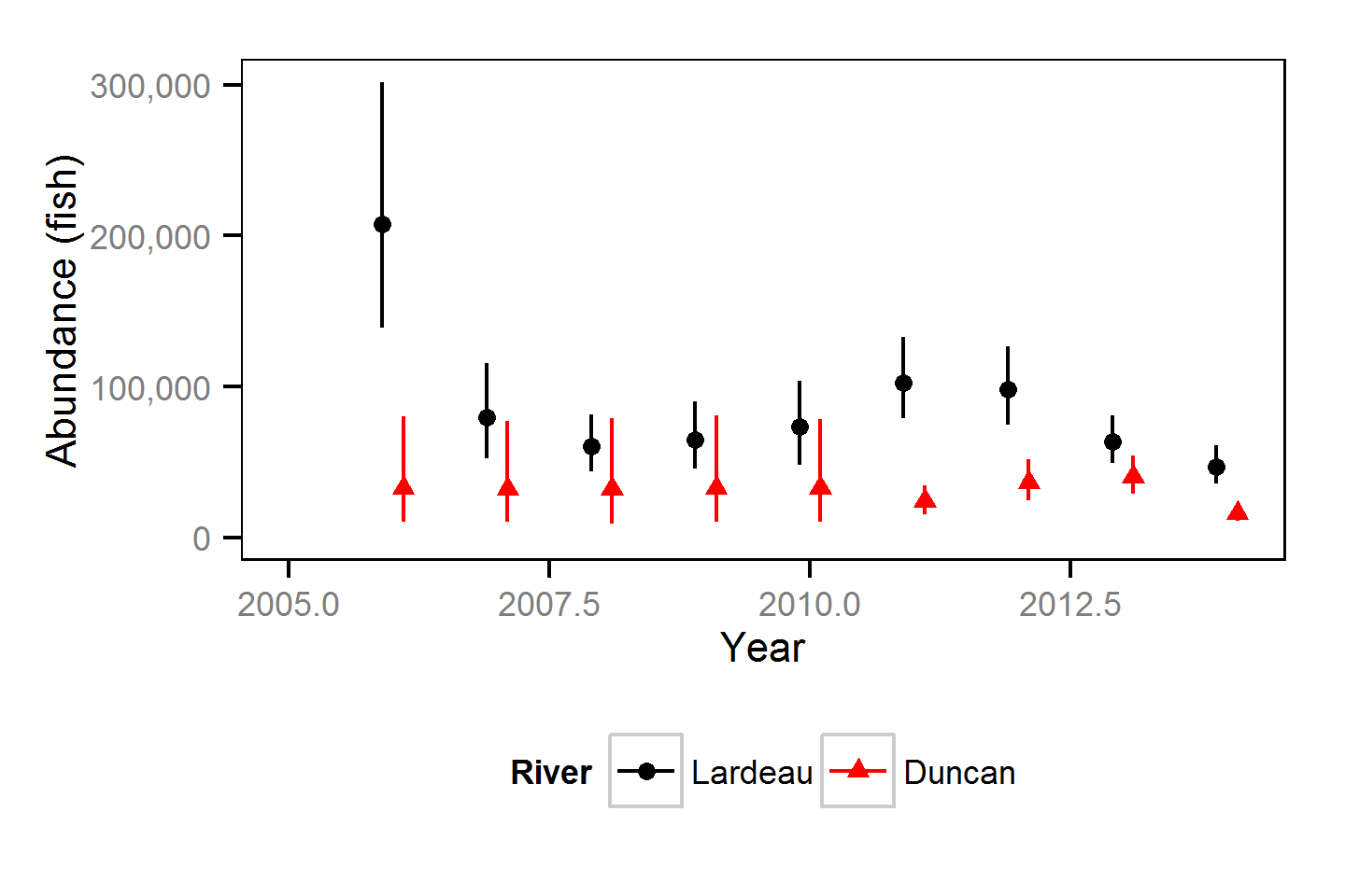
- Estimate the spring abundance of age-1 juvenile rainbow trout by year from snorkel survey data.
- Estimate the stock-recruitment relationship between the number of spawners at Gerrard and the number of age-1 juveniles the following spring.
Methods
Data Preparation
The snorkel count data was provided by Redfish Consulting Ltd. The Ministry of Forests, Lands and Natural Resource Operations (MFLNRO) provided the spawner escapement estimates for Gerrard.
Rainbow trout with a fork length \(\leq\) 100 mm are age-1.
Statistical Analysis
Hierarchical Bayesian models were fitted to the snorkel and stock-recruitment data using R version 3.1.0 (Team, 2013) and JAGS 3.4.0 (Plummer, 2012) which interfaced with each other via jaggernaut 1.8.2 (Thorley, 2014). For additional information on hierarchical Bayesian modelling in the BUGS language, of which JAGS uses a dialect, the reader is referred to Kery and Schaub (2011) pages 41-44.
Unless specified, the models assumed vague (low information) prior distributions (Kéry and Schaub, 2011, p. 36). The posterior distributions were estimated from a minimum of 1,000 Markov Chain Monte Carlo (MCMC) samples thinned from the second halves of three chains (Kéry and Schaub, 2011, pp. 38-40). Model convergence was confirmed by ensuring that Rhat (Kéry and Schaub, 2011, p. 40) was less than 1.1 for each of the parameters in the model (Kéry and Schaub, 2011, p. 61).
The posterior distributions of the fixed (Kéry and Schaub, 2011, p. 75) parameters are summarised in terms of a point estimate (mean), lower and upper 95% credible limits (2.5th and 97.5th percentiles), the standard deviation (SD), percent relative error (half the 95% credible interval as a percent of the point estimate) and significance (Kéry and Schaub, 2011, p. 37,42).
The results are displayed graphically by plotting the modeled relationships between particular variables and the response with 95% credible intervals (CRIs) with the remaining variables held constant. In general, continuous and discrete fixed variables are held constant at their mean and first level values respectively while random variables are held constant at their typical values (expected values of the underlying hyperdistributions) (Kéry and Schaub, 2011, pp. 77-82). Plots were produced using the ggplot2 R package (Wickham, 2009).
Abundance
The abundance was estimated using a mark-resight-based binomial mixture model (Kéry and Schaub, 2011, pp. 134-136,384-388).
Key assumptions of the abundance model include:
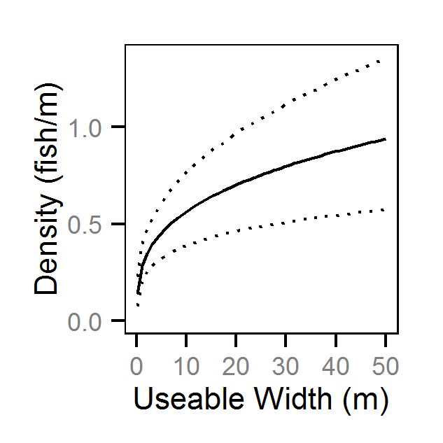
- Lineal density (fish/m) varies with useable width.
- Lineal density (fish/m) varies randomly with year within river and site.
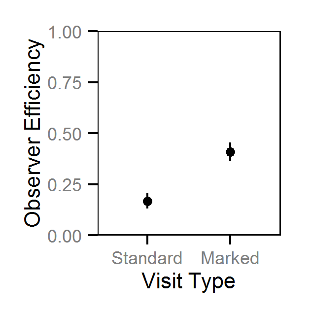
- Efficiency (probability of capture) varies by visit type (standard versus presence of marked fish).
- Marked and unmarked fish have the same probability of being counted.
- There is no tag loss, mortality or misidentification of fish.
- Sites are closed.
- The actual abundance at a site on a visit is described by an over-dispersed Poisson distribution- The number of marked and unmarked fish observed at a site are described by a binomial distributions.
Stock-Recruitment
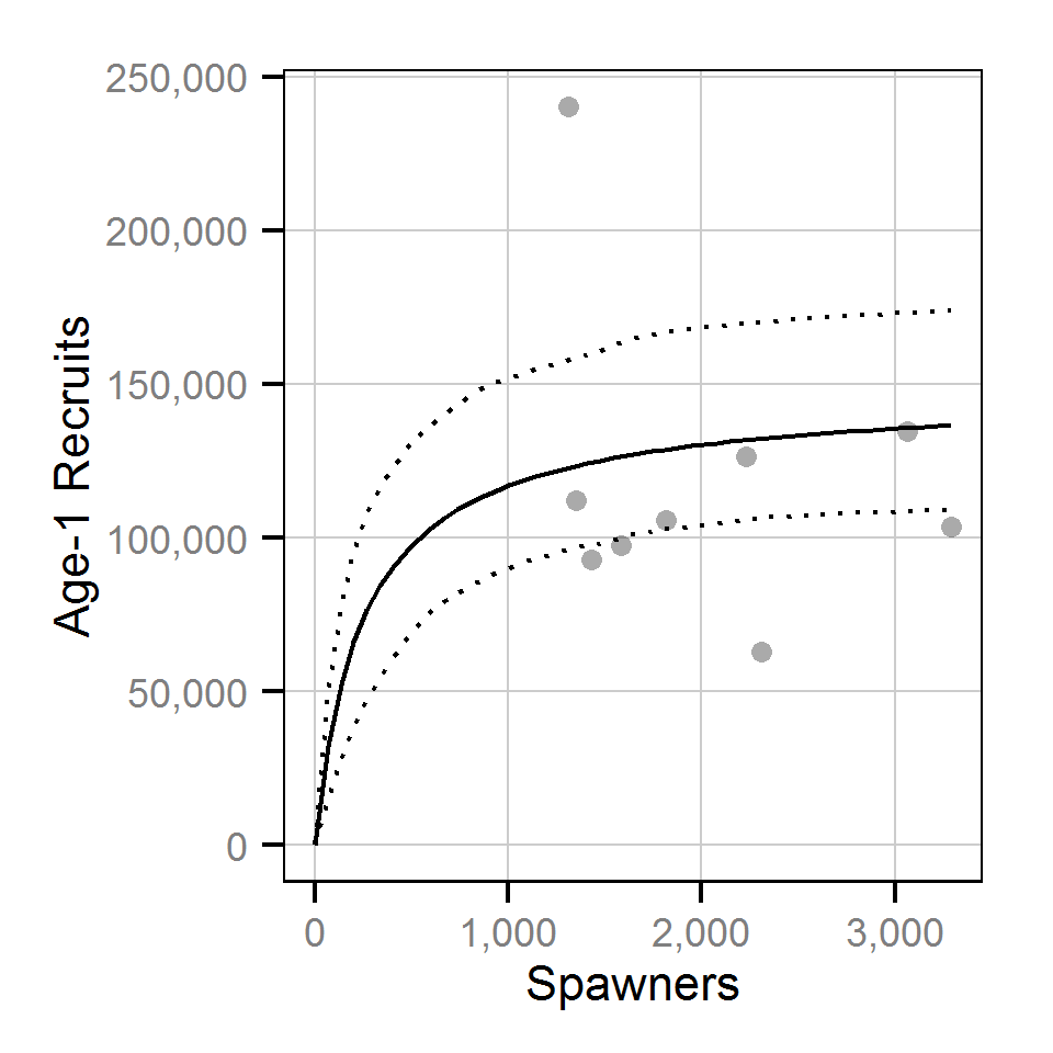
The relationship between the number of spawners and the number of age-1 recruits the following spring was estimated using a Beverton-Holt stock-recruitment model.
Key assumptions of the stock-recruitment model include:
- The prior probability for the number of recruits per spawner at low density (
R0) is normally distributed with a mean of 500 and a SD of 250. - The residual variation in the number of age-1 recruits is log-normally distributed.
The mean prior probability of 500 for R0 was based on an average of 8,000 eggs
per female spawner, a 50:50 sex ratio, 50% egg survival, 50% post-emergence fall survival
and 50% overwintering survival.
Model Code
The JAGS model code, which uses a series of naming conventions, is presented below.
Abundance
| Variable/Parameter | Description |
|---|---|
bDebsity0 |
Intercept for log(eDensity) |
bDensityRiverYear |
Effect of River within Year on log(eDensity) |
bDensitySite |
Effect of Site on log(eDensity) |
bDensityWidth |
Exponent for effect of Width on eDensity |
bEfficiency0 |
Intercept for logit(eEfficiency) |
bEfficiencyVisitType |
Effect of VisitType on logit(eEfficiency) |
eAbundance[ii] |
Expected abundance of fish at site of iith visit |
eDensity[ii] |
Expected desnity on iith visit |
eDispersion |
Overdispersion of eTotal |
eEfficiency[ii] |
Expected observer efficiency on the iith visit |
eTotal[ii] |
Expected total number of fish at site of iith visit |
Marked[ii] |
Number of fish marked prior to the iith visit |
Resighted[ii] |
Number of marked fish resighted during iith visit |
River[ii] |
River of iith visit |
sDensityRiverYear |
SD of effect of River within Year on log(eDensity) |
sDensitySite |
SD of effect of Site on log(eDensity) |
sDispersion |
SD of overdispersion term |
Site[ii] |
Site of iith visit |
SiteLength[ii] |
Length of site of iith visit |
SurveyProportion[ii] |
Proportion of site surveyed during iith visit |
Total[ii] |
Total number of fish observed during iith visit |
VisitType[ii] |
Visit type of iith visit |
Width[ii] |
Site width of iith visit |
Year[ii] |
Year of iith visit |
Abundance - Model1
model {

  bEfficiency0 ~ dnorm(0, 2^-2)

  bEfficiencyVisitType[1] <- 0
  for (vt in 2:nVisitType) {
    bEfficiencyVisitType[vt] ~ dnorm(0, 2^-2)
  }

  bDensity0 ~ dnorm(0, 5^-2)

  bDensityWidth ~ dnorm(0, 2^-2)

  sDensityRiverYear ~ dunif(0, 5)
  for (rv in 1:nRiver) {
    for (yr in 1:nYear) {
      bDensityRiverYear[rv, yr] ~ dnorm(0, sDensityRiverYear^-2)
    }
  }

  sDensitySite ~ dunif(0, 5)
  for (st in 1:nSite) {
    bDensitySite[st] ~ dnorm(0, sDensitySite^-2)
  }

  sDispersion ~ dunif(0, 5)

  for (ii in 1:length(Total)) {

    logit(eEfficiency[ii]) <- bEfficiency0
                            + bEfficiencyVisitType[VisitType[ii]]

    dEfficiencyMark[ii] <- min(eEfficiency[ii], Marked[ii])
    dMarked[ii] <- max(Marked[ii], 1)

    Resighted[ii] ~ dbin(dEfficiencyMark[ii], dMarked[ii])

    log(eDensity[ii]) <- bDensity0
                        + bDensityWidth * log(Width[ii])
                        + bDensityRiverYear[River[ii],Year[ii]]
                        + bDensitySite[Site[ii]]

    eAbundance[ii] <- eDensity[ii] * SiteLength[ii] * SurveyProportion[ii]

    eDispersion[ii] ~ dgamma(1/sDispersion^2, 1/sDispersion^2)
    eTotal[ii] ~ dpois(eAbundance[ii] * eDispersion[ii])

    Total[ii] ~ dbin(eEfficiency[ii], eTotal[ii])
  }
}
Stock Recruitment
| Variable/Parameter | Description |
|---|---|
eRecruits |
Expected number of age-1 recruits |
k |
Carrying capacity |
R0 |
Recruits per spawner at low density |
Recruits |
Number of age-1 recruits |
sRecruits |
SD of log-normally distributed residual variation in Recruits |
Stock |
Number of spawners at Gerrard |
Stock Recruitment - Model1
model {
  R0 ~ dnorm(8000 * 0.5^4, 250^-2) T(0,)
  k ~ dunif(5 * 10^4, 2.5 * 10^5)
  sRecruits ~ dunif(0, 5)

  for (ii in 1:length(Stock)) {
    eRecruits[ii] <- R0 * Stock[ii] / (1 + Stock[ii]*(R0-1)/k)

    Recruits[ii] ~ dlnorm(log(eRecruits[ii]), sRecruits^-2)
  }
}
Results
Model Parameters
The posterior distributions for the fixed (Kery and Schaub 2011 p. 75) parameters in each model are summarised below.
Abundance - Age-1
| Parameter | Estimate | Lower | Upper | SD | Error | Significance |
|---|---|---|---|---|---|---|
| bDensity0 | -1.3020 | -1.6317 | -0.9542 | 0.18145 | 26 | 0 |
| bDensityWidth | 0.3105 | 0.1995 | 0.4271 | 0.05996 | 37 | 0 |
| bEfficiency0 | -1.6203 | -1.8887 | -1.3539 | 0.14020 | 17 | 0 |
| bEfficiencyVisitType[2] | 1.2524 | 0.9872 | 1.5151 | 0.13688 | 21 | 0 |
| sDensityRiverYear | 0.4737 | 0.2959 | 0.7711 | 0.12388 | 50 | 0 |
| sDensitySite | 0.7688 | 0.6718 | 0.8687 | 0.05104 | 13 | 0 |
| sDispersion | 0.9029 | 0.8399 | 0.9689 | 0.03210 | 7 | 0 |
| Rhat | Iterations |
|---|---|
| 1.09 | 64000 |
Stock Recruitment
| Parameter | Estimate | Lower | Upper | SD | Error | Significance |
|---|---|---|---|---|---|---|
| k | 1.323e+05 | 1.053e+05 | 1.50e+05 | 1.121e+04 | 17 | 0 |
| R0 | 5.720e+02 | 2.278e+02 | 1.01e+03 | 2.034e+02 | 68 | 0 |
| sRecruits | 4.344e-01 | 2.521e-01 | 7.64e-01 | 1.415e-01 | 59 | 0 |
| Rhat | Iterations |
|---|---|
| 1.03 | 1e+05 |
Figures
Abundance
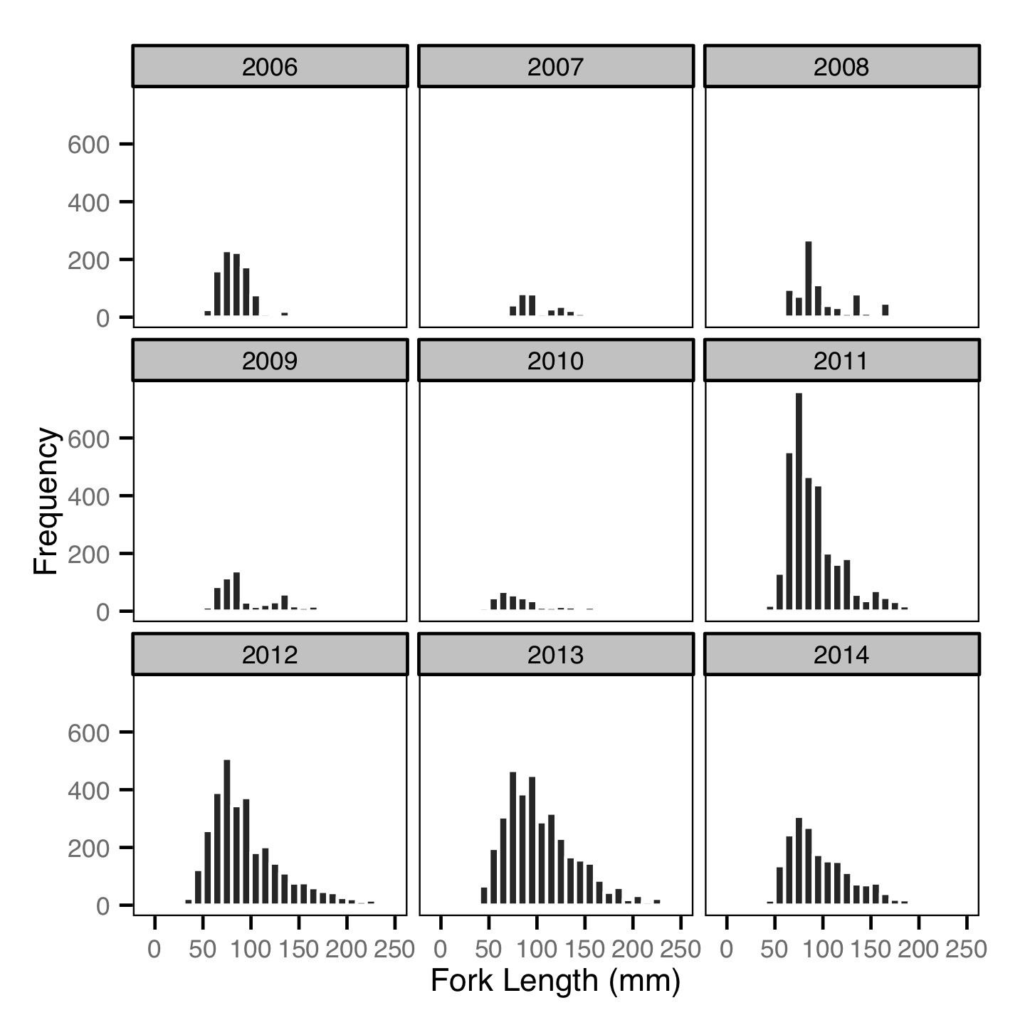
Abundance - Age-1
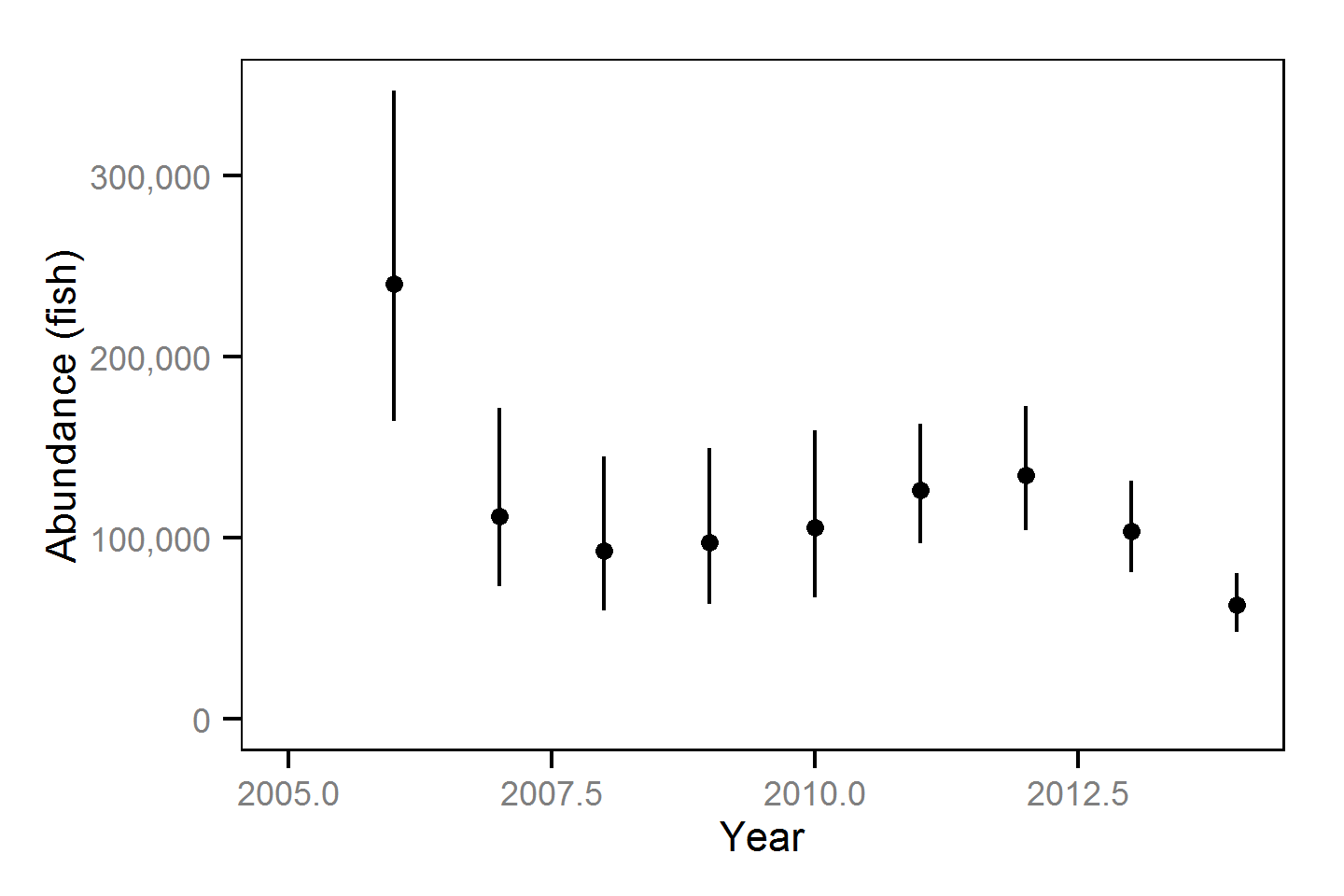
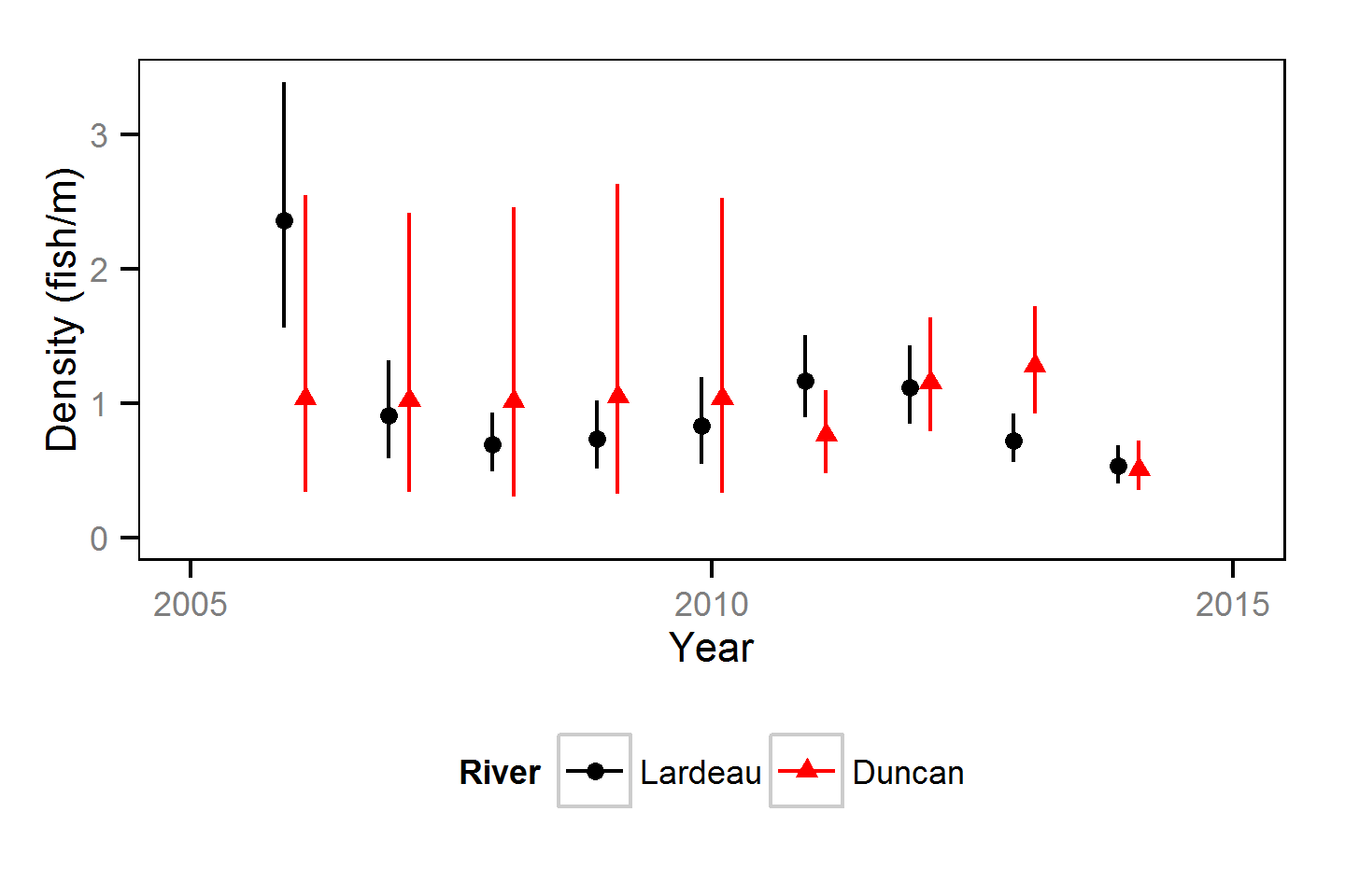
Stock Recruitment
References
- {G.F.} Andrusak, (2013) Determination of Gerrard Rainbow Trout Productivity and Capacity in Defining Management Reference Points: Progress Report. http://a100.gov.bc.ca/pub/acat/public/viewReport.do?reportId=36011
- Hadley Wickham, (2009) ggplot2: elegant graphics for data analysis. http://had.co.nz/ggplot2/book
- Joseph Thorley, (2014) jaggernaut: An R package to facilitate Bayesian analyses using JAGS (Just Another Gibbs Sampler). https://github.com/joethorley/jaggernaut
- Marc Kéry, Michael Schaub, (2011) Bayesian population analysis using {WinBUGS} : a hierarchical perspective. http://www.vogelwarte.ch/bpa.html
- Martyn Plummer, (2012) {JAGS} version 3.3.0 user manual. http://sourceforge.net/projects/mcmc-jags/files/Manuals/3.x/
- R Team, (2013) R: a language and environment for statistical computing. http://www.R-project.org
Acknowledgements
The organisations and individuals whose contributions have made this analysis report possible include: - Habitat Conservation Trust Foundation (HCTF) and the anglers, hunters, trappers and guides who contribute to the Trust - Fish and Wildlife Compensation Program (FWCP) and its program partners BC Hydro, the Province of BC and Fisheries and Oceans Canada - Ministry of Forests, Lands and Natural Resource Operations (MFLNRO) - Redfish Consulting - Greg Andrusak - Gary Pavan