Lardeau-Lower Duncan River Juvenile Rainbow Trout Abundance and Stock-Recruitment Analysis 2016
The suggested citation for this analytic report is:
Thorley, J.L. and Hogan, P.M. (2016) Lardeau-Lower Duncan River Juvenile Rainbow Trout Abundance and Stock-Recruitment 2016. A Poisson Consulting Analysis Report. URL: https://www.poissonconsulting.ca/f/6848898.
Background
Juvenile Age-1 Gerrard Rainbow Trout from Kootenay Lake rear in the Lardeau and Lower Duncan rivers. From 2006 to 2014 and in 2016 spring snorkel surveys were done to estimate the abundance of Age-1 fish. From 2006 and 2010 the surveys were conducted at fixed index site. From 2010 fish observations were mapped to sites on the river by georeferencing all counts which allowed the swimmers to cover more of the river.
The primary aims of the current analyses are to:
- Estimate the observer efficiency when conducting spring snorkel surveys for Age-1 fish.
- Estimate the spring abundance of Age-1 fish by year.
- Estimate the stock-recruitment relationship between the number of spawners in a given year and the number of Age-1 recruits the following spring.
Methods
Data Preparation
The snorkel count data was provided by Redfish Consulting Ltd. The Ministry of Forests, Lands and Natural Resource Operations (MFLNRO) provided the AUC-based spawner escapement estimates for Gerrard.
Length-Bias Correction
Biases in length estimation were estimated manually; for each observer for each unique day of observations, a fork-length cut-off between Age-1 and Age-2+ fish was estimated, which was then used to classify each fish by lifestage.
Statistical Analysis
Hierarchical Bayesian models were fitted to the data using R version 3.2.4 (R Core Team 2015) and JAGS 4.2.0 (Plummer 2015) which interfaced with each other via jaggernaut 2.3.2 (Thorley 2013). For additional information on hierarchical Bayesian modelling in the BUGS language, of which JAGS uses a dialect, the reader is referred to (Kery and Schaub 2011, 41–44).
Unless specified, the models assumed vague (low information) prior distributions (Kery and Schaub 2011, 36). The posterior distributions were estimated from a minimum of 1,000 Markov Chain Monte Carlo (MCMC) samples thinned from the second halves of three chains (Kery and Schaub 2011, 38–40). Model convergence was confirmed by ensuring that Rhat (Kery and Schaub 2011, 40) was less than 1.1 for each of the parameters in the model (Kery and Schaub 2011, 61).
The posterior distributions of the fixed (Kery and Schaub 2011, 75) parameters are summarised in terms of a point estimate (mean), lower and upper 95% credible limits (2.5th and 97.5th percentiles), the standard deviation (SD), percent relative error (half the 95% credible interval as a percent of the point estimate) and significance (Kery and Schaub 2011, 37, 42).
Variable selection was achieved by dropping insignificant (Kery and Schaub 2011, 37, 42) fixed (Kery and Schaub 2011, 77–82) variables and uninformative random variables. A fixed variable was considered to be insignificant if its significance was \(\geq\) 0.05 while a random variable was considered to be uninformative if its percent relative error was \(\geq\) 80%. The Deviance Information Criterion (DIC) was not used because it is of questionable validity when applied to hierarchical models (Kery and Schaub 2011, 469).
The results are displayed graphically by plotting the modelled relationships between particular variables and the response with 95% credible intervals (CRIs) with the remaining variables held constant. In general, continuous and discrete fixed variables are held constant at their mean and first level values respectively while random variables are held constant at their typical values (expected values of the underlying hyperdistributions) (Kery and Schaub 2011, 77–82). Where informative the influence of particular variables is expressed in terms of the effect size (i.e., percent change in the response variable) with 95% CRIs (Bradford, Korman, and Higgins 2005).
Observer Efficiency
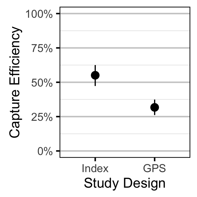
The observer efficiency for Age-1 fish was estimated using a mark-resight binomial model (Kery and Schaub 2011, 134–36, 384–88).
Key assumptions of the observer efficiency model include:
- The observer probability varies with study design (Index and GPS).
- There is no tag loss.
- There is no emigration of marked fish.
- The number of marked fish that are resighted is described by a binomial distribution.
Abundance
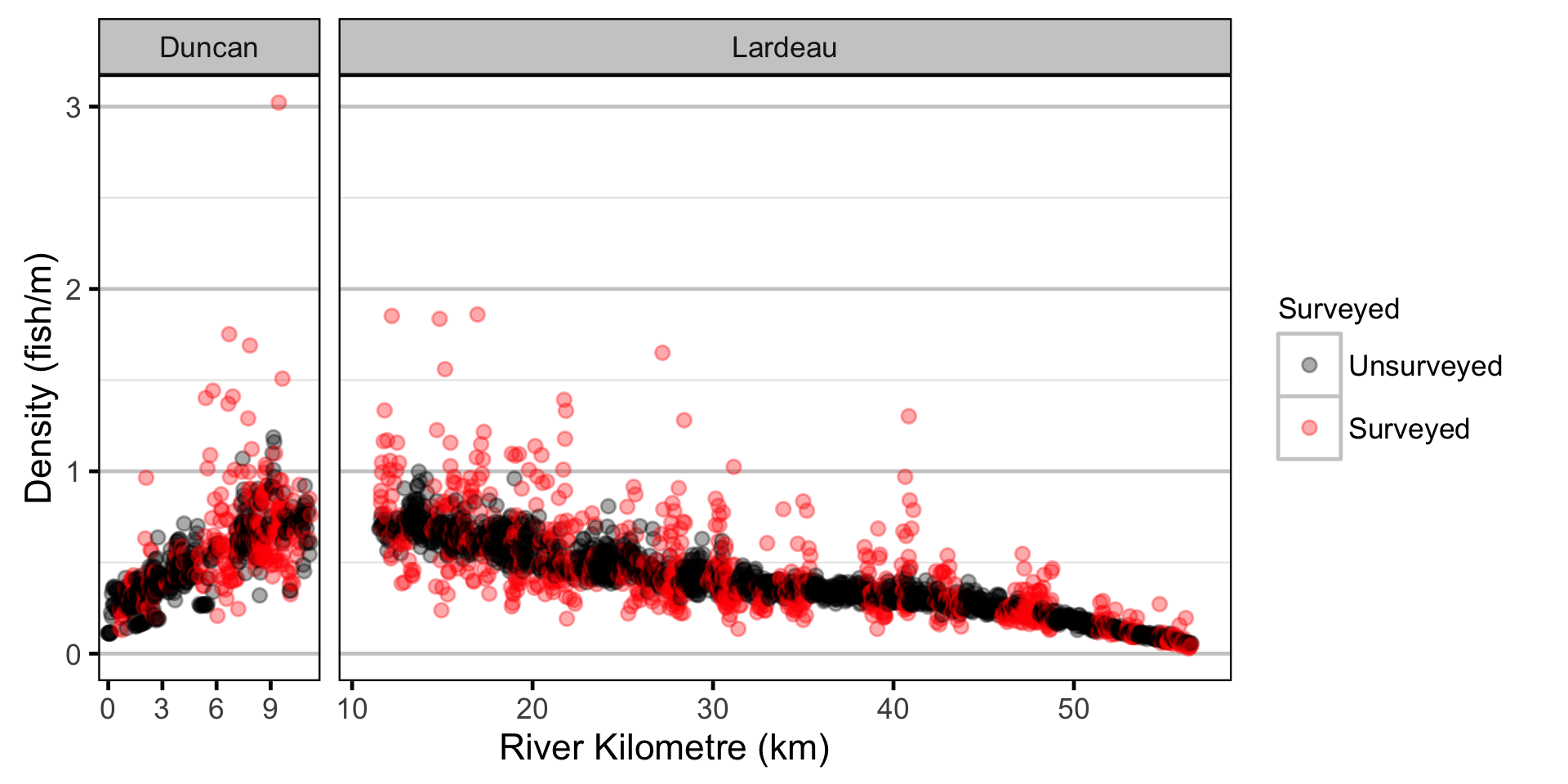
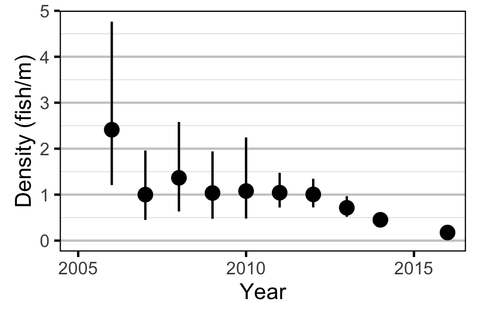
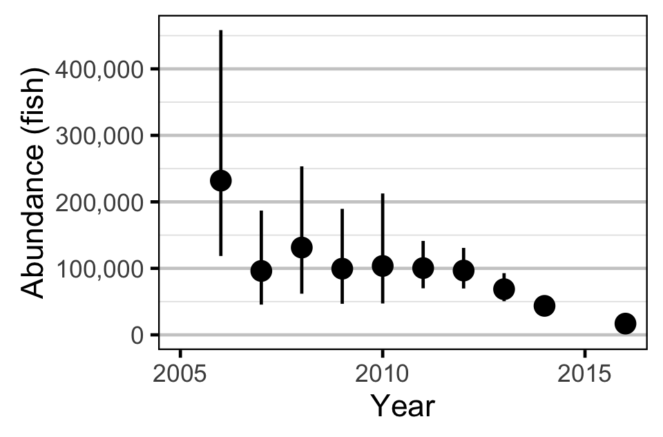
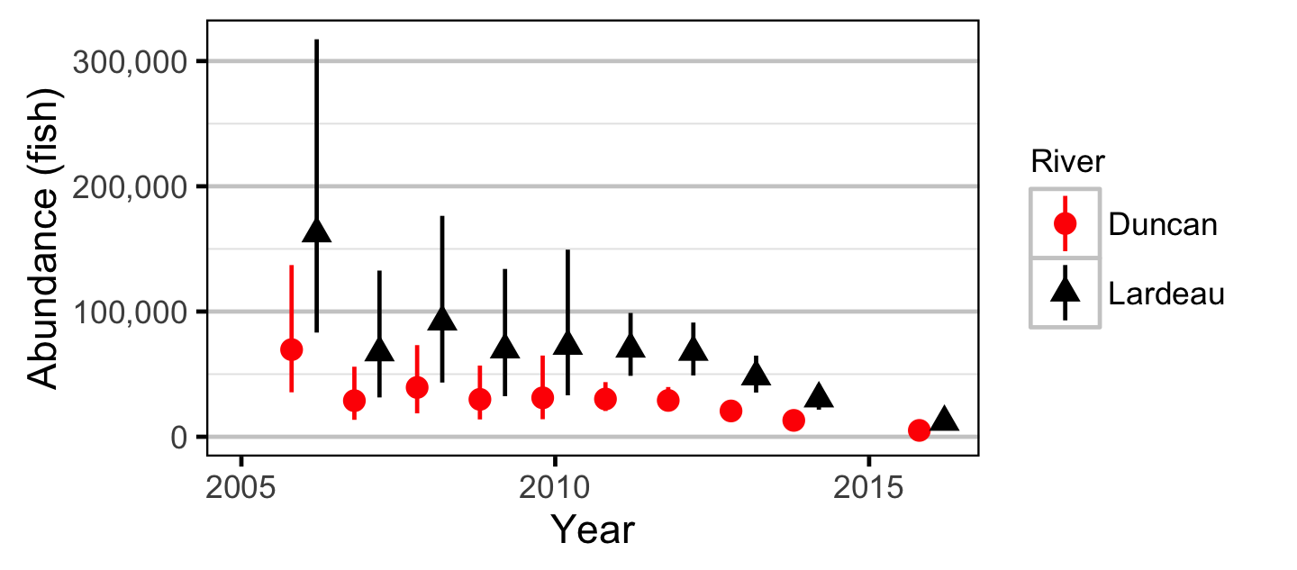
The abundance was estimated from the length bias-corrected observer count data using an overdispersed Poisson model (Kery and Schaub 2011, 55–56). The annual abundance estimates represent the total number of fish in the study area.
Key assumptions of the abundance model include:
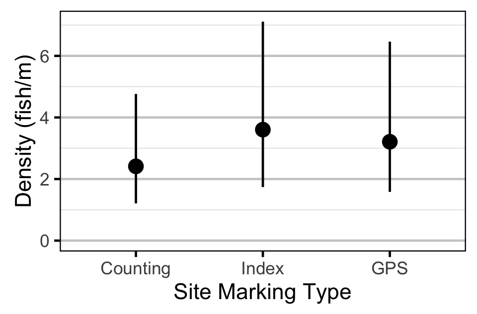
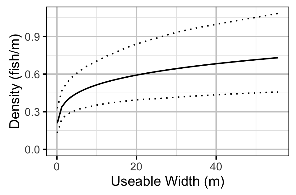
- The lineal fish density varies with year, useable width and river kilometer as a polynomial, and randomly with site.
- The observer efficiency at marked sites was as estimated by the observer efficiency model (which varied by study design).
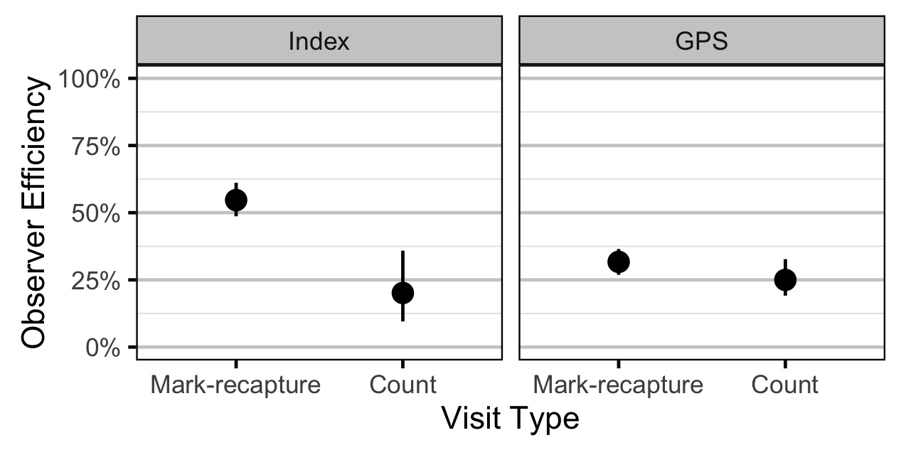
- The observer efficiency also varies with visit type (standard count versus presence of marked fish) within study design, and randomly with swimmer.
- The expected count at a site is the expected lineal density multiplied by the site length, the observer efficiency and the proportion of the site surveyed.
- The residual variation in the actual count, which is gamma-Poisson distributed, varies with the annual lineal fish density.
Stock-Recruitment
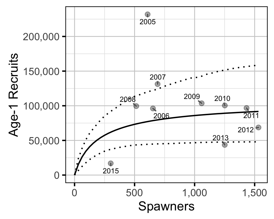
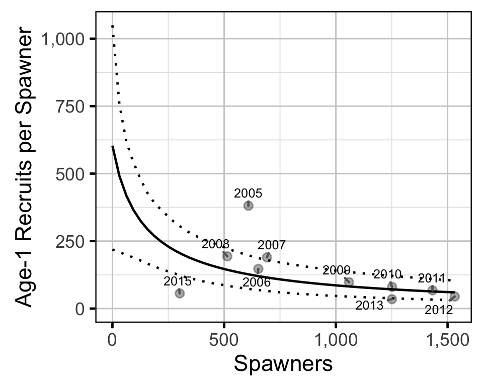
The relationship between the number of spawners in a given year (\(S\)) and the number of Age-1 recruits the following spring (\(R\)) was estimated using a Bayesian Beverton-Holt stock-recruitment model (Walters and Martell 2004):
\[ R = \frac{a \cdot S}{1 + b \cdot S} \quad,\]
where \(a\) is the maximum reproductive performance per spawner, and \(b\) determines the population size scaling.
Key assumptions of the stock-recruitment model include:
- The prior probability \(a\) is normally distributed with a mean of 500 and a SD of 250; this mean is based on an average of 8,000 eggs per female spawner, a 50:50 sex ratio, 50% egg survival, 50% post-emergence fall survival and 50% overwintering survival.
- The residual variation in the number of recruits is log-normally distributed.
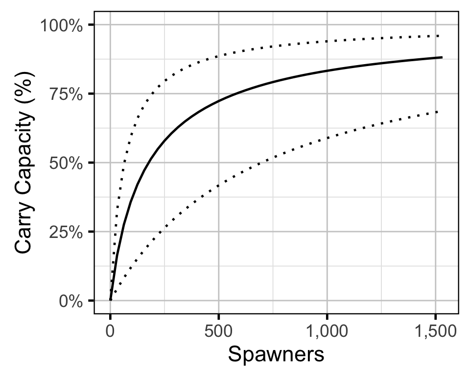
We may determine the maximum recruit population \(K\) that the environment can sustain indefinitely, the carrying capacity, by the relation:
\[ K = \frac{a}{b} \quad.\]
Model Code
The JAGS model code, which uses a series of naming conventions, is presented below.
Capture Efficiency
| Variable/Parameter | Description |
|---|---|
bEfficiency |
logit(eEfficiency) intercept |
bEfficiencyStudyDesign[ii] |
Effect of iith study design on logit(eEfficiency) |
eEfficiency[ii] |
Expected capture efficiency on iith visit |
Marked[ii] |
Number of marked fish prior to iith visit |
Resighted[ii] |
Number of marked fish resighted on iith visit |
StudyDesign[ii] |
Study design of iith visit |
Capture Efficiency - Model1
model{

  bEfficiency ~ dnorm(0, 5^-2)

  bEfficiencyStudyDesign[1] <- 0
  for (ii in 2:nStudyDesign) {
    bEfficiencyStudyDesign[ii] ~ dnorm(0, 2^-2)
  }

  for(ii in 1:length(Marked)){
    logit(eEfficiency[ii]) <- bEfficiency
                            + bEfficiencyStudyDesign[StudyDesign[ii]]

    Resighted[ii] ~ dbin(eEfficiency[ii], Marked[ii])
  }
}
Abundance
| Variable/Parameter | Description |
|---|---|
bDensityMarking |
Effect of Marking on log(eDensity) |
bDensityRkmX |
Polynomial coefficients of effect of river kilometer on log(eDensity) |
bDensitySite[ii] |
Effect of iith site on log(eDensity) |
bDensityWidth |
Effect of site width on log(eDensity) |
bDensityYear[yr] |
Estimate of log(eDensity) for yrth year |
bEfficiencySwimmer[ii] |
Effect of iith swimmer on logit(eEfficiency) |
bEfficiencyVisitStudy[ii, jj] |
Effect of iith visit type within jjth study design on logit(eEfficiency) |
bSDispersion0 |
Estimate of log(eSDispersion) |
bSDispersion1 |
Effect of bDensityYear on log(eSDispersion) |
eAbundance[ii] |
Expected abundance of fish at site of iith visit |
eCount[ii] |
Expected total number of fish at site of iith visit |
eDensity[ii] |
Expected lineal density of fish at site of iith visit |
eDispersion[ii] |
Expected overdispersion of Count[ii] |
eEfficiency[ii] |
Expected observer efficiency on iith visit |
eSDispersion[ii] |
Expected SD of overdispersion of Count[ii] |
logit(bEfficiencyStudy[ii]) |
Effect of iith study design on logit(eEfficiency) |
Marking |
Whether a site has been chosen as a marking site under the different study designs |
Rkm[ii] |
River kilometer of iith visit |
sDensitySite |
SD of effect of site on log(eDensity) |
sEfficiencySwimmer |
SD of effect of swimmer on logit(eEfficiency) |
Site[ii] |
Site of iith visit |
SiteLength[ii] |
Length of site of iith visit |
StudyDesign[ii] |
Study design of iith visit |
SurveyProportion[ii] |
Proportion of site surveyed on iith visit |
Swimmer[ii] |
Swimmer of iith visit |
VisitType[ii] |
Visit type of iith visit |
Width[ii] |
Site width of iith visit |
Year[ii] |
Year of iith visit |
Abundance - Model1
model{
    for(yr in 1:nYear){
    bDensityYear[yr] ~ dnorm(0, 5^-2)
  }

    bDensityWidth ~ dnorm(0, 2^-2)

    sDensitySite ~ dunif(0, 5)
  for(st in 1:nSite){
    bDensitySite[st] ~ dnorm(-sDensitySite^2 / 2, sDensitySite^-2)
  }

  bDensityMarking[1] <- 0
  for(mk in 2:nMarking) {
    bDensityMarking[mk] ~ dnorm(0, 5^-2)
  }

    sEfficiencySwimmer ~ dunif(0, 5)
  for(sw in 1:nSwimmer){
    bEfficiencySwimmer[sw] ~ dnorm(0, sEfficiencySwimmer^-2)
  }

    bDensityRkm1 ~ dnorm(0, 2^-2)
  bDensityRkm2 ~ dnorm(0, 2^-2)
  bDensityRkm3 ~ dnorm(0, 2^-2)
  bDensityRkm4 ~ dnorm(0, 2^-2)

    for(sd in 1:nStudyDesign){
    bEfficiencyStudy[sd] ~ dnorm(Efficiency[sd], Efficiency.sd[sd]^-2) T(Efficiency.lower[sd], Efficiency.upper[sd])
  }

    for(sd in 1:nStudyDesign){
    bEfficiencyVisitStudy[1, sd] <- 0
    for(vt in 2:nVisitType){
      bEfficiencyVisitStudy[vt, sd] ~ dnorm(0, 2^-2)
    }
  }

    bSDispersion0 ~ dnorm(0, 2^-2)
  bSDispersion1 ~ dnorm(0, 2^-2)

    for(ii in 1:length(Count)){
    log(eDensity[ii]) <- bDensityYear[Year[ii]]
                       + bDensityWidth * log(Width[ii])
                       + bDensitySite[Site[ii]]
                       + bDensityRkm1 * Rkm[ii]
                       + bDensityRkm2 * Rkm[ii]^2
                       + bDensityRkm3 * Rkm[ii]^3
                       + bDensityRkm4 * Rkm[ii]^4
                       + bDensityMarking[Marking[ii]]

    eAbundance[ii] <- eDensity[ii] * SiteLength[ii]

    logit(eEfficiency[ii]) <- logit(bEfficiencyStudy[StudyDesign[ii]])
                            + bEfficiencyVisitStudy[VisitType[ii], StudyDesign[ii]]
                            + bEfficiencySwimmer[Swimmer[ii]]

    eCount[ii] <- eAbundance[ii] * eEfficiency[ii] * SurveyProportion[ii]

    log(eSDispersion[ii]) <- bSDispersion0 + bSDispersion1 * bDensityYear[Year[ii]]

    eDispersion[ii] ~ dgamma(1/eSDispersion[ii]^2, 1/eSDispersion[ii]^2)

    Count[ii] ~ dpois(eCount[ii] * eDispersion[ii])
  }
}
Stock-Recruitment
| Variable/Parameter | Description |
|---|---|
a |
Maximum reproductive performance per spawner |
b |
Population size scaling parameter |
eRecruits[i] |
Expected number of recruits in ith spawn year |
Recruits[i] |
Number of recruits in ith spawn year |
Spawners[i] |
Number of spawners in ith spawn year |
sRecruits |
Standard deviation of residual variation in log(eRecruits) |
Stock-Recruitment - Model1
model {

  a ~ dnorm(8000 * 0.5^4, 250^-2) T(0, )
  b ~ dunif(0, 0.1)

  sRecruits ~ dunif(0, 5)

  for(i in 1:length(Spawners)){
    eRecruits[i] <- a * Spawners[i] / (1 + Spawners[i] * b)
    Recruits[i] ~ dlnorm(log(eRecruits[i]), sRecruits^-2)
  }
}
Results
Stock-Recruitment
The maximum reproductive performance per spawner was estimated to be 603 (219 - 1050 95% CRI).
The environmental recruit carrying capacity was estimated to be 107,000 (50,500 - 211,200 95% CRI).
Model Parameters
The posterior distributions for the fixed (Kery and Schaub 2011 p. 75) parameters in each model are summarised below.
Capture Efficiency - Fry
| Parameter | Estimate | Lower | Upper | SD | Error | Significance |
|---|---|---|---|---|---|---|
| bEfficiency | 0.2055 | -0.1089 | 0.5121 | 0.1565 | 150 | 0.1807 |
| bEfficiencyStudyDesign[2] | -0.9755 | -1.3770 | -0.5923 | 0.2051 | 40 | 0.0010 |
| Convergence | Iterations |
|---|---|
| 1 | 5000 |
Abundance - Fry
| Parameter | Estimate | Lower | Upper | SD | Error | Significance |
|---|---|---|---|---|---|---|
| bDensityMarking[2] | 0.39970 | 0.0605 | 0.71770 | 0.16650 | 82 | 0.0232 |
| bDensityMarking[3] | 0.28220 | 0.0804 | 0.49100 | 0.10640 | 73 | 0.0097 |
| bDensityRkm1 | -0.47620 | -0.6462 | -0.31540 | 0.08600 | 35 | 0.0010 |
| bDensityRkm2 | 0.28750 | 0.0482 | 0.50670 | 0.11830 | 80 | 0.0155 |
| bDensityRkm3 | 0.05130 | -0.0258 | 0.13300 | 0.04090 | 160 | 0.2068 |
| bDensityRkm4 | -0.19750 | -0.2750 | -0.11640 | 0.04110 | 40 | 0.0010 |
| bDensityWidth | 0.19940 | 0.0923 | 0.29220 | 0.05150 | 50 | 0.0010 |
| bDensityYear[1] | -0.20800 | -0.8540 | 0.52800 | 0.34700 | 330 | 0.5392 |
| bDensityYear[10] | -2.78120 | -3.1332 | -2.44960 | 0.18230 | 12 | 0.0010 |
| bDensityYear[2] | -1.09200 | -1.7830 | -0.36700 | 0.36100 | 65 | 0.0020 |
| bDensityYear[3] | -0.77700 | -1.4610 | -0.07000 | 0.34800 | 90 | 0.0310 |
| bDensityYear[4] | -1.05900 | -1.7700 | -0.34100 | 0.36200 | 68 | 0.0020 |
| bDensityYear[5] | -1.02900 | -1.7700 | -0.23700 | 0.39200 | 75 | 0.0097 |
| bDensityYear[6] | -1.00100 | -1.3650 | -0.62590 | 0.18860 | 37 | 0.0010 |
| bDensityYear[7] | -1.03520 | -1.3712 | -0.69060 | 0.17940 | 33 | 0.0010 |
| bDensityYear[8] | -1.37640 | -1.6902 | -1.05010 | 0.16990 | 23 | 0.0010 |
| bDensityYear[9] | -1.83290 | -2.1605 | -1.48350 | 0.17540 | 18 | 0.0010 |
| bEfficiencyStudy[1] | 0.54680 | 0.4866 | 0.61120 | 0.03260 | 11 | 0.0010 |
| bEfficiencyStudy[2] | 0.31698 | 0.2688 | 0.36487 | 0.02528 | 15 | 0.0010 |
| bEfficiencyVisitStudy[2,1] | -1.61300 | -2.4710 | -0.78400 | 0.40800 | 52 | 0.0010 |
| bEfficiencyVisitStudy[2,2] | -0.33710 | -0.6132 | -0.02040 | 0.15150 | 88 | 0.0387 |
| bSDispersion0 | 0.03960 | -0.1712 | 0.29640 | 0.11250 | 590 | 0.7208 |
| bSDispersion1 | 0.16260 | 0.0140 | 0.34770 | 0.08210 | 100 | 0.0329 |
| sDensitySite | 0.59180 | 0.4957 | 0.68120 | 0.04600 | 16 | 0.0010 |
| sEfficiencySwimmer | 0.44080 | 0.2471 | 0.76430 | 0.13670 | 59 | 0.0010 |
| Convergence | Iterations |
|---|---|
| 1.05 | 20000 |
Stock-Recruitment
| Parameter | Estimate | Lower | Upper | SD | Error | Significance |
|---|---|---|---|---|---|---|
| a | 603.30000 | 218.90000 | 1049.60000 | 213.70000 | 69 | 0.001 |
| b | 0.00663 | 0.00143 | 0.01555 | 0.00382 | 110 | 0.001 |
| sRecruits | 0.79030 | 0.47830 | 1.39130 | 0.22950 | 58 | 0.001 |
| Convergence | Iterations |
|---|---|
| 1 | 5e+05 |
Figures
Capture Efficiency - Fry
Abundance - Fry
Stock-Recruitment
Acknowledgements
The organisations and individuals whose contributions have made this analysis report possible include:
- Habitat Conservation Trust Foundation (HCTF) and the anglers, hunters, trappers and guides who contribute to the Trust.
- Fish and Wildlife Compensation Program (FWCP) and its program partners BC Hydro, the Province of BC and Fisheries and Oceans Canada.
- Ministry of Forests, Lands and Natural Resource Operations (MFLNRO)
- Redfish Consulting
- Greg Andrusak
- Gary Pavan
References
Bradford, Michael J, Josh Korman, and Paul S Higgins. 2005. “Using Confidence Intervals to Estimate the Response of Salmon Populations (Oncorhynchus Spp.) to Experimental Habitat Alterations.” Canadian Journal of Fisheries and Aquatic Sciences 62 (12): 2716–26. https://doi.org/10.1139/f05-179.
Kery, Marc, and Michael Schaub. 2011. Bayesian Population Analysis Using WinBUGS : A Hierarchical Perspective. Boston: Academic Press. http://www.vogelwarte.ch/bpa.html.
Plummer, Martyn. 2015. “JAGS Version 4.0.1 User Manual.” http://sourceforge.net/projects/mcmc-jags/files/Manuals/4.x/.
R Core Team. 2015. “R: A Language and Environment for Statistical Computing.” Vienna, Austria: R Foundation for Statistical Computing. http://www.R-project.org/.
Thorley, J. L. 2013. “Jaggernaut: An R Package to Facilitate Bayesian Analyses Using JAGS (Just Another Gibbs Sampler).” Nelson, B.C.: Poisson Consulting Ltd. https://github.com/poissonconsulting/jaggernaut.
Walters, Carl J., and Steven J. D. Martell. 2004. Fisheries Ecology and Management. Princeton, N.J: Princeton University Press.