Horse Lake Exploitation Analysis 2020

2021-02-18

The suggested citation for this analytic appendix is:

Thorley, J.L., Dalgarno, S. & Pearson, A. (2021) Horse Lake Exploitation Analysis 2020. A Poisson Consulting Analysis Appendix. URL: https://www.poissonconsulting.ca/f/1065913173.

Background

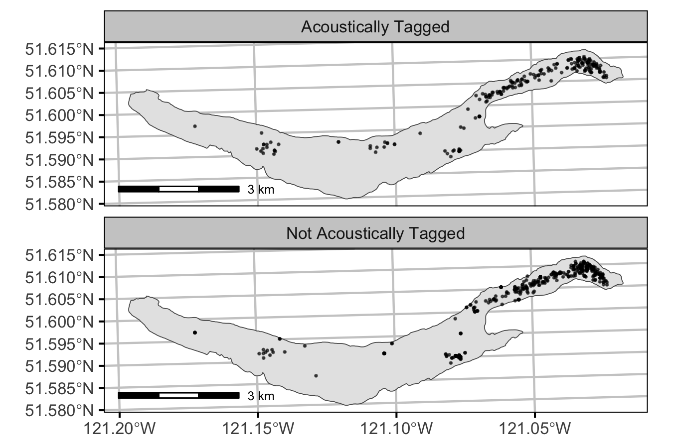
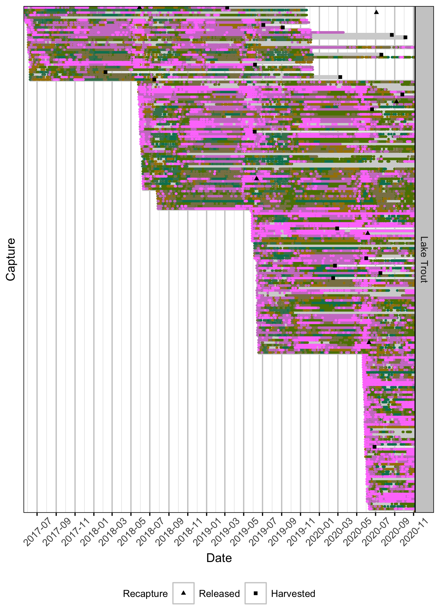
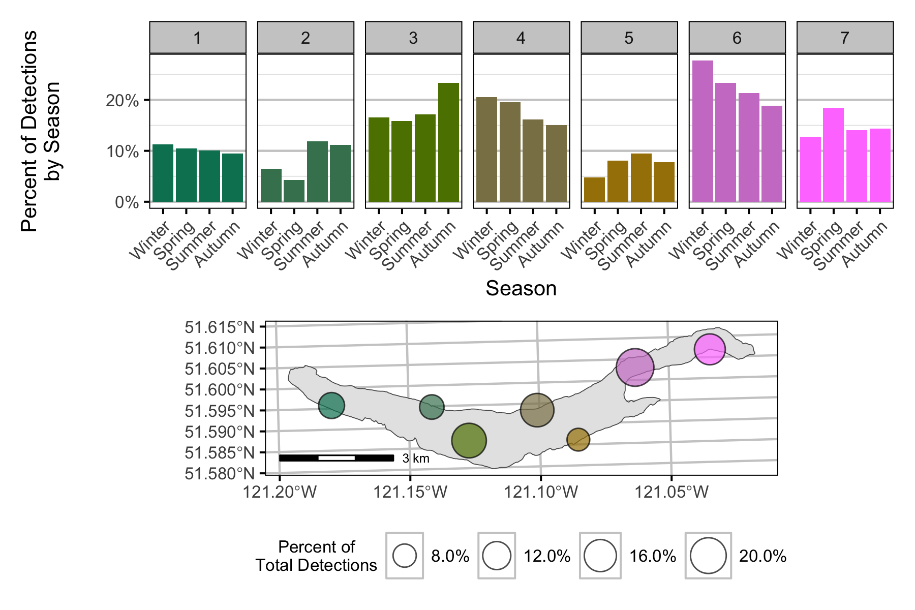
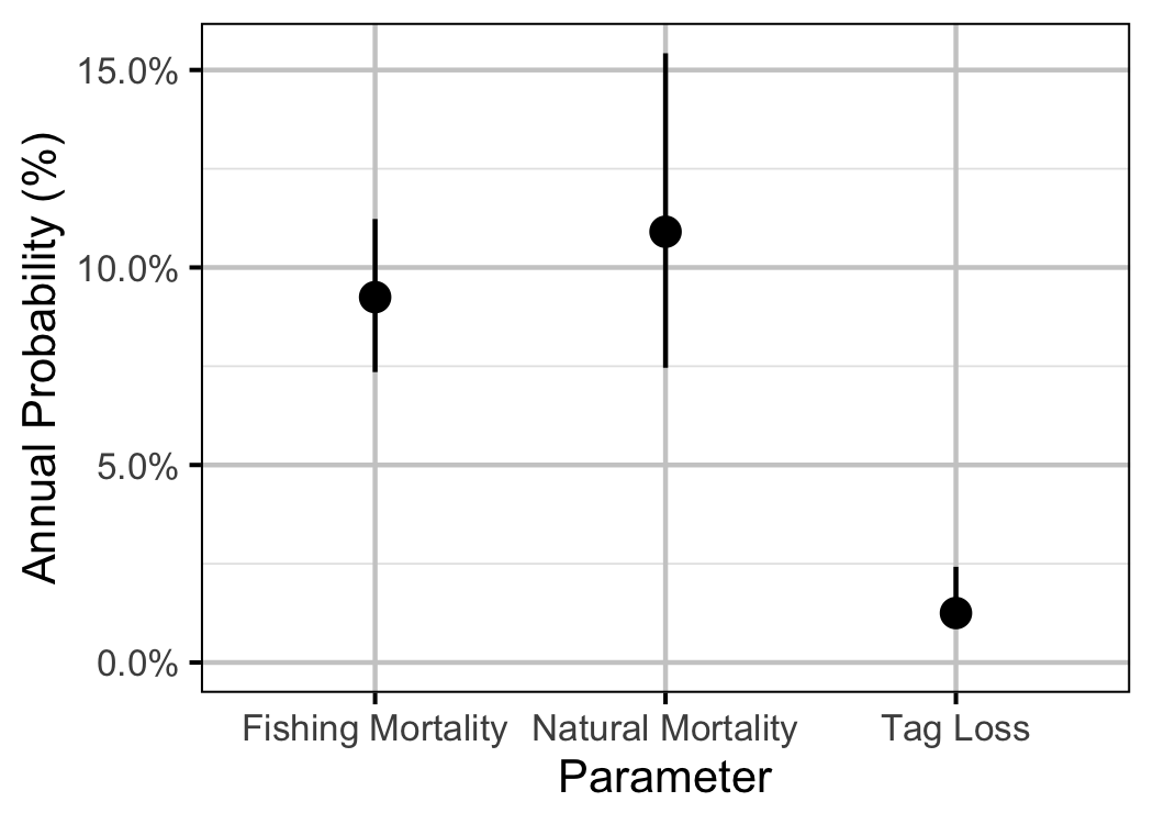
Horse Lake supports a recreational fishery for Lake Trout (Salvelinus namaycush). To estimate their natural and fishing mortality, individuals were caught by angling and tagged with acoustic transmitters and/or external reward tags. Acoustically tagged fish were detected by a series of seven receivers distributed through the lake as well as annual mobile receiver surveys. The external reward tags included a phone number for anglers to report their recaptures. In 2019, eight Rainbow Trout with acoustic transmitters and external reward tags were transplanted from Greenlee Lake.

All the data were provided by the Ministry of Forests, Lands and Natural Resource Operations (MFLNRO) Cariboo Region.

Methods

Data Preparation

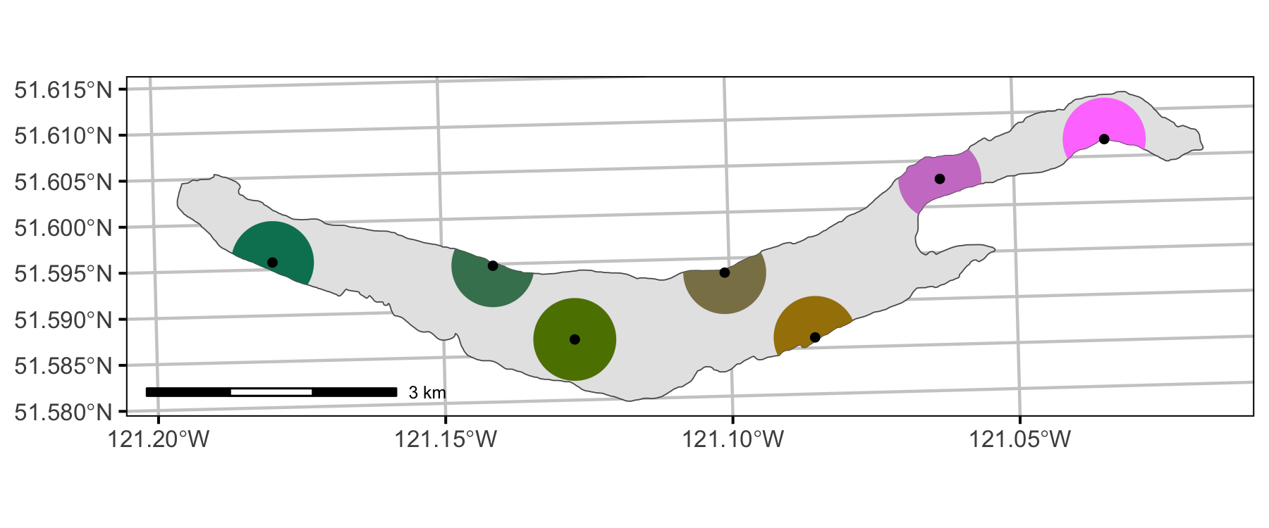
The data were prepared for analysis using R version 4.0.4 (R Core Team 2020). Receivers were assumed to have a detection range of 500 m. Detections were aggregated daily, where for each transmitter the receiver with the most detections was chosen. In the case of a tie, the receiver with the greatest coverage area was chosen.

The Seasons were Winter (December - February), Spring (March - May), Summer (June - August) and Autumn (September - November).

Data Analysis

Hierarchical Bayesian models were fitted to the data using R version 4.0.4 (R Core Team 2020) and JAGS 4.2.0 (Plummer 2015) which interfaced with each other via the jmbr package. For additional information on hierarchical Bayesian modelling in the BUGS language, of which JAGS uses a dialect, the reader is referred to Kery and Schaub (2011, 41–44).

Unless stated otherwise, the Bayesian analyses used weakly informative normal and half-normal prior distributions (Gelman, Simpson, and Betancourt 2017). The posterior distributions were estimated from 1500 Markov Chain Monte Carlo (MCMC) samples thinned from the second halves of 3 chains (Kery and Schaub 2011, 38–40). Model convergence was confirmed by ensuring that the potential scale reduction factor $\hat{R} \leq 1.05$ (Kery and Schaub 2011, 40) and the effective sample size (Brooks et al. 2011) $\textrm{ESS} \geq 150$ for each of the monitored parameters (Kery and Schaub 2011, 61).

The parameters are summarised in terms of the point estimate, lower and upper 95% credible limits (CLs) and the surprisal s-value (Greenland 2019). The estimate is the median (50th percentile) of the MCMC samples while the 95% CLs are the 2.5th and 97.5th percentiles. The s-value can be considered a test of directionality. More specifically it indicates how surprising (in bits) it would be to discover that the true value of the parameter is in the opposite direction to the estimate. An s-value of 4.3 bits, which is equivalent to a p-value (Kery and Schaub 2011; Greenland and Poole 2013) of 0.05, indicates that the surprise would be equivalent to throwing 4.3 heads in a row. The condition that non-essential explanatory variables have s-values $\geq$ 4.3 bits provides a useful model selection heuristic (Kery and Schaub 2011).

The results are displayed graphically by plotting the modeled relationships between particular variables and the response with the remaining variables held constant. In general, continuous and discrete fixed variables are held constant at their mean and first level values respectively while random variables are held constant at their typical values (expected values of the underlying hyperdistributions) (Kery and Schaub 2011, 77–82). Where informative the influence of particular variables is expressed in terms of the effect size (i.e., percent change in the response variable) with 95% CIs (Bradford, Korman, and Higgins 2005).

Model Descriptions

Condition

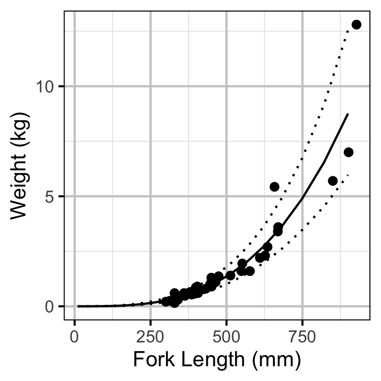
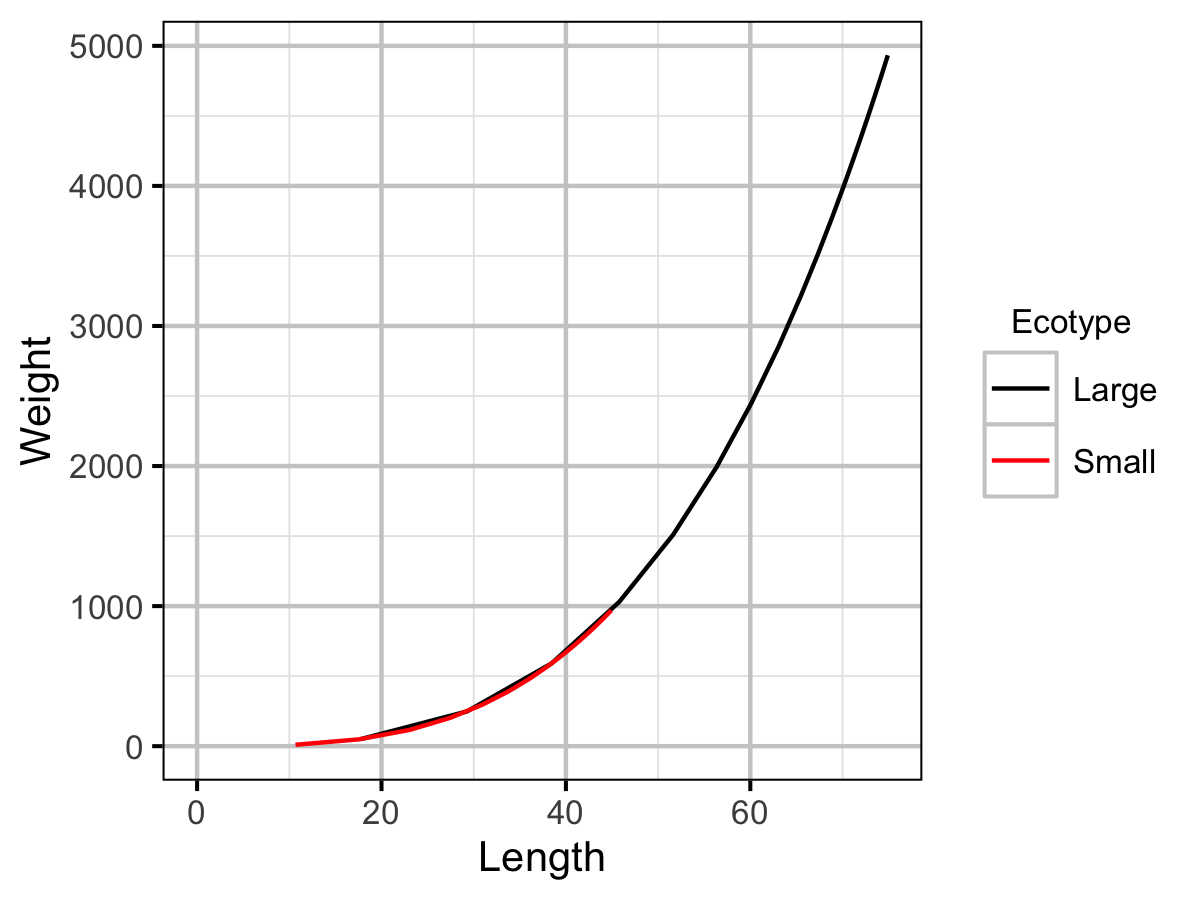
The expected weight of a fish of a given length was estimated from the data using an allometric mass-length model (He et al. 2008)

\[ L = \alpha W^\beta\]

Key assumptions of the condition model include:

The prior distribution on the power term ($\beta$) is a normal distribution with a mean of 3.18 and a standard deviation of 0.19 (McDermid, Shuter, and Lester 2010).
The residual variation in weight is log-normally distributed.

Growth

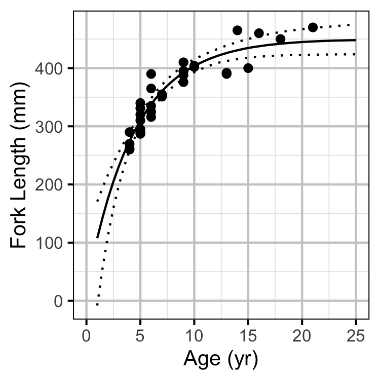
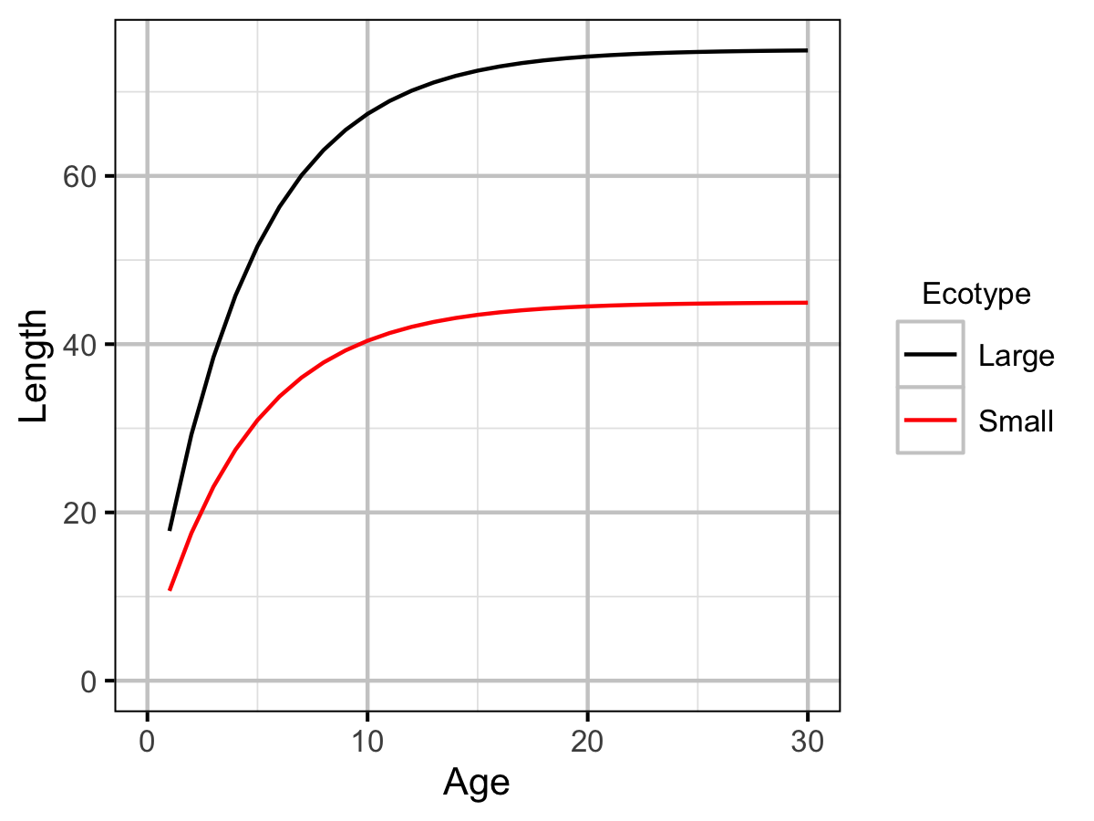
Growth was estimated from length and scale age data for Horse Lake using a Von Bertalanffy growth curve model (von Bertalanffy 1938).

\[ L = L_\infty \cdot (1 - \exp(-k \cdot (A - t_0) ))\]

where $A$ is the scale age in years and $t_0$ is the extrapolated age at zero length.

Key assumptions of the growth model include:

The residual variation in length is normally distributed.

1 fish with a fork length $\geq$ 500 mm was excluded from the analysis.

Survival

The natural mortality and capture probability for individuals $\geq$ 300 mm was estimated using a Bayesian individual state-space survival model (Thorley and Andrusak 2017) with monthly intervals. The survival model incorporated natural and handling mortality, acoustic detection, movement, T-bar tag loss, recapture and reporting. Key assumptions of the survival model include:

The tagged individuals are a random sample from the population.
The only effects of tagging are change in the natural mortality for three months following acoustic tagging.
The prior probability on the annual interval individual external tag loss rate is a uniform distribution between 1 and 30% (Fabrizio et al. 1996).
All individuals are correctly identified.
There is no emigration out of the lake.
There are no unmodelled individual differences in the probability of recapture in each time interval.
There are no unmodelled individual differences in the probability of survival in each time interval.
There are no unmodelled individual differences in the probability of a living individual with an active acoustic transmitter being detected moving among sections in each time period.
The fate of each individual is independent of the fate of any other individual.
The sampling periods are instantaneous and all individuals are immediately released.

The survival model treats all recaptured fish as if they had been retained. Only individuals with a fork length (FL) $\geq$ 300 mm that were tagged with an acoustic tag and/or $100 and $10 reward tags were included in the survival analysis. Preliminary analysis indicated that the difference between the natural mortality and fishing mortality rates for individuals $\geq$ 500 mm were not sigificant.

Yield-Per-Recruit

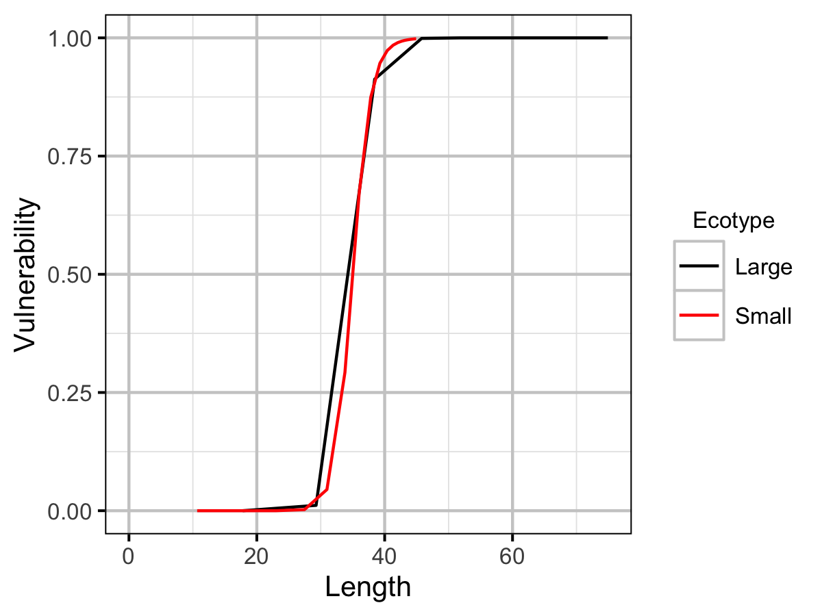
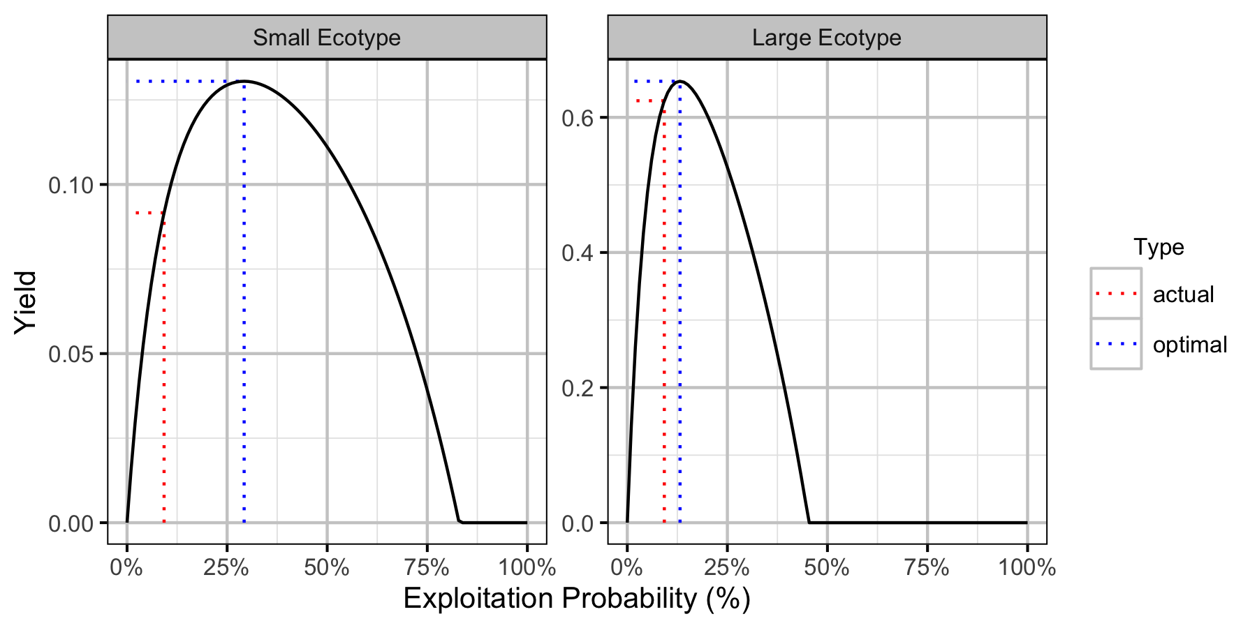
The optimal capture rate (to maximize biomass harvested assuming 100% retention) was calculated using yield-per-recruit analysis (Walters and Martell 2004). A separate yield-per-recruit analysis was performed for the two different Lake Trout ecotypes in Horse Lake.

Results

Templates

Condition

.model {
  bWeight ~ dnorm(0, 1^-2) 
  bWeightLength ~ dnorm(3.18, 0.19^-2)

  sWeight ~ dnorm(0, 1^-2) T(0,) 
  for(i in 1:length(LogLength)) {
    eWeight[i] <- bWeight + bWeightLength * LogLength[i]
    Weight[i] ~ dlnorm(eWeight[i], exp(sWeight)^-2)
  }

Block 1. Condition model description.

Growth

.model {
  bLInf ~ dnorm(500, 100^-2) T(0, )
  bK ~ dnorm(0, 1^-2) T(0, )
  bT0 ~ dnorm(0, 1^-1)

  sLength ~ dnorm(0, 100^-2) T(0, )
  for (i in 1:length(Length)) {
    eLength[i] <- bLInf * (1 - exp(-bK * (Age[i] - bT0))) 
    Length[i] ~ dnorm(eLength[i], sLength^-2) T(0, )
  }

Block 2. Growth model description.

Survival

.model{
  bMortality ~ dnorm(-3, 3^-2)
  bMortalityHandling ~ dnorm(0, 2^-2)
  bTagLoss ~ dunif(1 - (1 - 0.01)^(1/12), 1 - (1 - 0.30)^(1/12))
  bDetected ~ dunif(0, 1)
  bMoved ~ dunif(0, 1)
  bRecaptured ~ dunif(0, 1 - (1 - 0.50)^(1/12))
  bReported ~ dunif(0.9, 1.00)

  for (i in 1:nCapture){
    logit(eMortality[i,PeriodCapture[i]]) <- bMortality + bMortalityHandling
    eTagLoss[i,PeriodCapture[i]] <- bTagLoss
    eDetected[i,PeriodCapture[i]] <- bDetected
    eMoved[i,PeriodCapture[i]] <- bMoved
    eRecaptured[i,PeriodCapture[i]] <- bRecaptured
    eReported[i,PeriodCapture[i]] <- bReported
    InLake[i,PeriodCapture[i]] <- 1
    Alive[i,PeriodCapture[i]] ~ dbern(1-eMortality[i,PeriodCapture[i]])
    TBarTag100[i,PeriodCapture[i]] ~ dbern(1-eTagLoss[i,PeriodCapture[i]])
    TBarTag10[i,PeriodCapture[i]] ~ dbern(1-eTagLoss[i,PeriodCapture[i]])
    Detected[i,PeriodCapture[i]] ~ dbern(Monitored[i,PeriodCapture[i]] * eDetected[i,PeriodCapture[i]])
    Moved[i,PeriodCapture[i]] ~ dbern(Alive[i,PeriodCapture[i]] * Monitored[i,PeriodCapture[i]] * eMoved[i,PeriodCapture[i]])
    Recaptured[i,PeriodCapture[i]] ~ dbern(Alive[i,PeriodCapture[i]] * eRecaptured[i,PeriodCapture[i]])
    Reported[i,PeriodCapture[i]] ~ dbern(Recaptured[i,PeriodCapture[i]] * eReported[i,PeriodCapture[i]] * step(TBarTag100[i,PeriodCapture[i]] + TBarTag10[i,PeriodCapture[i]] - 1))
  for(j in (PeriodCapture[i]+1):nPeriod) {
    logit(eMortality[i,j]) <- bMortality + bMortalityHandling * step(PeriodCapture[i] - j + 2)
    eTagLoss[i,j] <- bTagLoss
    eDetected[i,j] <- bDetected
    eMoved[i,j] <- bMoved
    eRecaptured[i,j] <- bRecaptured
    eReported[i,j] <- bReported
    InLake[i,j] ~ dbern(InLake[i,j-1] * (1-Recaptured[i,j-1]))
    Alive[i,j] ~ dbern(Alive[i,j-1] * (1-Recaptured[i,j-1]) * (1-eMortality[i,j-1]))
    TBarTag100[i,j] ~ dbern(TBarTag100[i,j-1] * (1-Recaptured[i,j-1]) * (1-eTagLoss[i,j]))
    TBarTag10[i,j] ~ dbern(TBarTag10[i,j-1] * (1-Recaptured[i,j-1]) * (1-eTagLoss[i,j]))
    Detected[i,j] ~ dbern(InLake[i,j] * Monitored[i,j] * eDetected[i,j])
    Moved[i,j] ~ dbern(Alive[i,j] * Monitored[i,j] * eMoved[i,j])
    Recaptured[i,j] ~ dbern(Alive[i,j] * eRecaptured[i,j])
    Reported[i,j] ~ dbern(Recaptured[i,j] * eReported[i,j] * step(TBarTag100[i,j] + TBarTag10[i,j] - 1))}}
  }

Block 3. Survival model description.

Tables

Captures

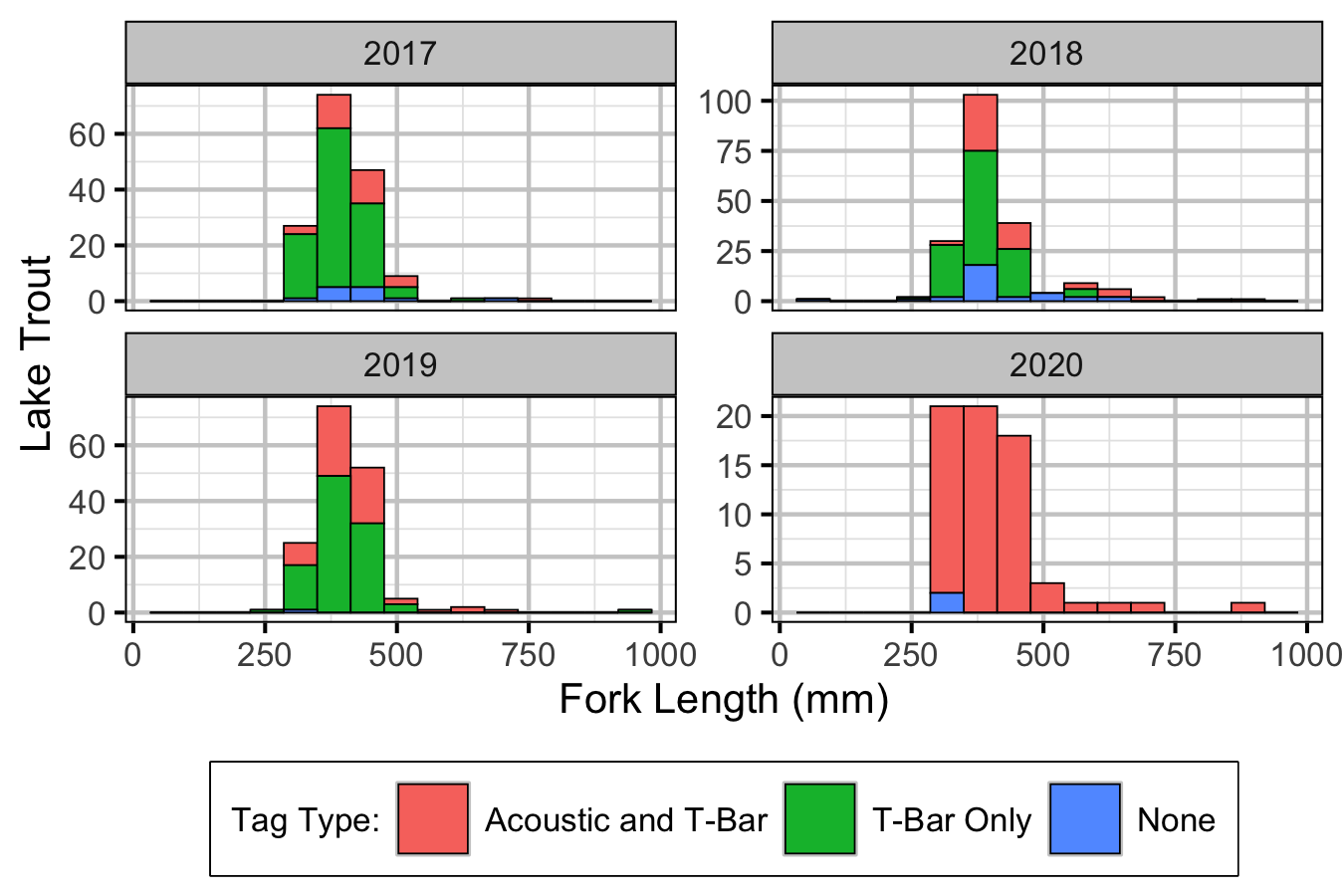
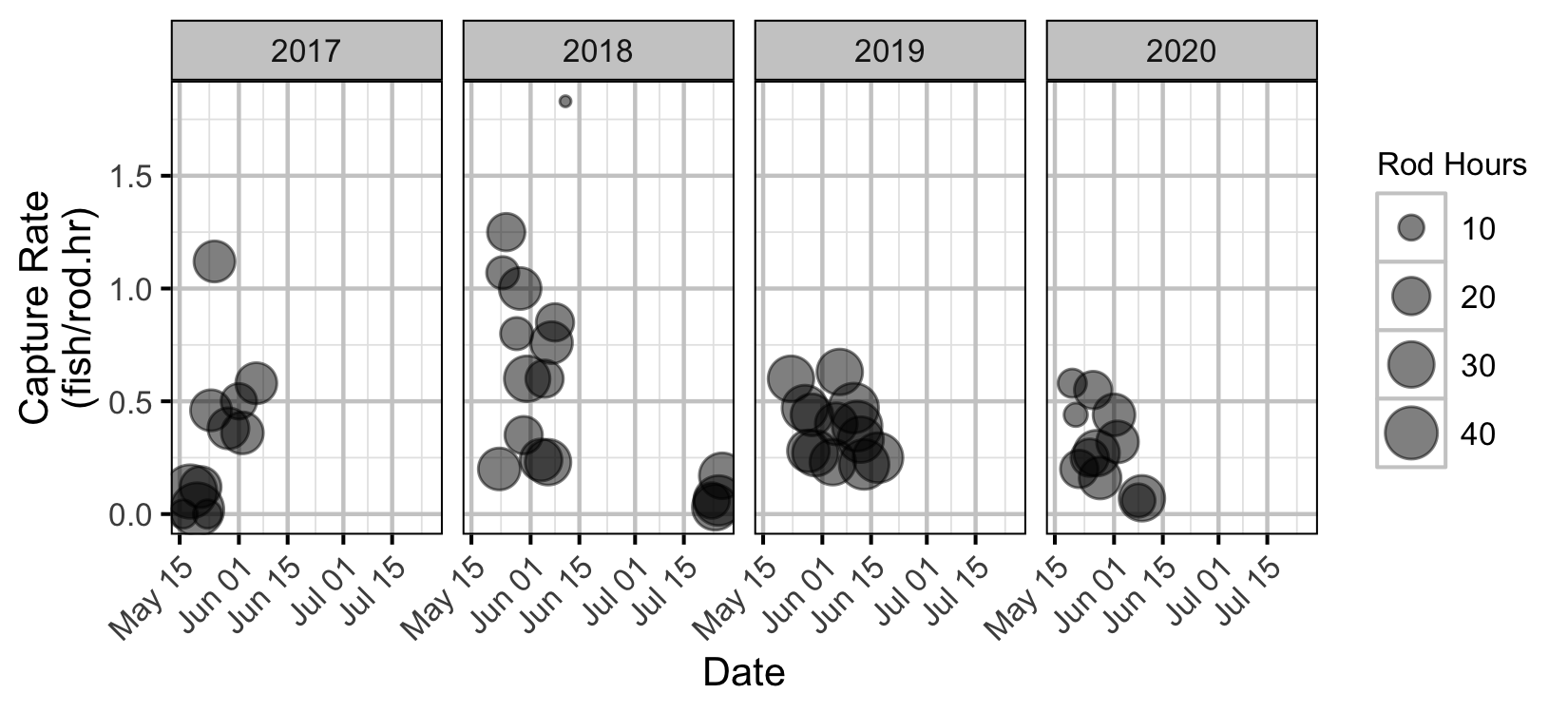
Table 1. Number of fish captured by year, species and size class. Eight Rainbow Trout were transplanted in 2019. Four fish were removed from previous captured totals as they were recaptures.

Year	Species	< 300 mm	300 - 500 mm	>= 500 mm	Total
2017	Kokanee	3	20	0	23
2017	Lake Trout	1	152	7	160
2017	Rainbow Trout	0	3	0	3
2018	Kokanee	0	2	0	2
2018	Lake Trout	4	175	19	198
2019	Lake Trout	3	152	7	162
2019	Rainbow Trout	0	8	0	8
2020	Lake Trout	0	61	6	67
Total		11	573	39	623

Table 2. Number of Lake Trout captured by size class, and tag class. Any fish > 500mm is classified as ‘large.’ Four fish were removed from previous captured totals as they were recaptures.

Year	Size	Acoustic and T-Bar	T-Bar Only	No Tag	Total
2017	< 300 mm	0	1	0	1
2017	300 - 500 mm	29	112	11	152
2017	>= 500 mm	3	2	2	7
2018	< 300 mm	0	2	2	4
2018	300 - 500 mm	43	106	26	175
2018	>= 500 mm	11	4	4	19
2019	< 300 mm	0	3	0	3
2019	300 - 500 mm	55	96	1	152
2019	>= 500 mm	4	3	0	7
2020	300 - 500 mm	59	0	2	61
2020	>= 500 mm	6	0	0	6
Total		210	329	48	587

Recaptures

Table 3. All Lake Trout recaptures to date. Recaptures with natural mortality were tags found in the stomach of another fish!.

Date Capture	Fork Length (mm)	Date Recapture	External Tag Number 1	External Tag Number 2	Harvested	Natural Mortality
2017-06-06	445	2017-07-07	278	544	Yes	No
2017-05-20	405	2017-09-08	86	337	Yes	No
2017-06-01	441	2018-01-29	289	532	Yes	No
2017-05-31	385	2018-02-02	441	NA	Yes	No
2017-06-07	439	2018-02-08	258	413	Yes	No
2018-05-25	400	2018-05-28	2315	1390	Yes	No
2017-05-18	360	2018-05-29	76	326	No	No
2018-05-29	379	2018-05-29	151	445	No	No
2018-05-25	436	2018-06-28	2316	1391	Yes	No
2018-05-30	341	2018-07-03	2370	NA	Yes	Yes
2018-06-11	406	2018-07-03	136	552	Yes	Yes
2017-05-21	370	2018-07-05	89	340	Yes	No
2017-06-07	416	2018-07-16	251	404	Yes	No
2018-05-25	334	2018-07-18	2320	1395	Yes	No
2018-05-30	416	2018-07-24	2368	1335	No	No
2017-06-02	360	2018-09-10	538	NA	No	No
2018-05-31	411	2019-01-15	2386	362	Yes	No
2018-06-08	382	2019-01-25	2340	377	Yes	No
2017-05-18	360	2019-03-09	76	326	Yes	No
2018-06-07	325	2019-03-09	2327	390	Yes	No
2017-05-30	402	2019-03-31	56	512	No	No
2018-06-11	411	2019-05-07	140	556	Yes	No
2019-05-23	421	2019-05-23	129	462	No	No
2018-05-29	356	2019-06-06	2354	1347	Yes	No
2017-06-01	421	2019-06-06	291	530	Yes	No
2017-05-29	429	2019-06-06	70	523	Yes	No
2017-06-06	405	2019-06-07	275	547	Yes	No
2017-06-06	343	2019-06-11	270	424	Yes	No
2018-05-28	421	2019-06-11	221	1321	No	No
2018-06-07	386	2019-06-12	2326	391	No	No
2018-06-11	410	2019-07-01	137	553	Yes	No
2017-05-29	425	2019-07-01	65	519	Yes	No
2017-05-30	480	2019-07-04	167	429	Yes	No
2019-05-23	377	2019-07-06	46	596	Yes	No
2018-06-11	407	2019-07-07	142	558	Yes	No
2018-06-08	394	2019-07-15	149	565	Yes	No
2018-05-25	395	2019-07-22	2321	1396	Yes	No
2018-10-24	592	2019-07-28	134	466	Yes	No
2019-06-06	349	2019-08-13	186	1490	Yes	No
2019-06-06	500	2019-09-04	187	1491	Yes	No
2017-05-31	450	2019-09-05	201	500	Yes	No
2018-05-29	415	2019-09-05	210	1310	Yes	No
2019-06-06	418	2020-01-26	196	1500	Yes	No
2019-06-11	433	2020-02-15	1958	1437	Yes	No
2018-06-04	404	2020-02-15	2376	358	Yes	No
2018-06-08	408	2020-02-15	2350	566	Yes	No
2017-05-31	386	2020-02-15	165	431	Yes	No
2018-06-08	385	2020-02-16	2342	575	Yes	No
2019-06-11	409	2020-02-21	1963	1442	Yes	No
2019-05-23	418	2020-02-21	133	600	Yes	No
2018-05-29	346	2020-02-22	2366	1337	Yes	No
2017-05-24	415	2020-02-25	19	319	Yes	No
2018-05-29	360	2020-02-27	2362	1341	Yes	No
2019-05-27	434	2020-02-28	29	457	Yes	No
2017-06-07	395	2020-03-09	405	NA	Yes	No
2019-06-10	414	2020-03-23	181	1485	Yes	No
2018-06-07	412	2020-04-04	2335	382	Yes	No
2019-05-29	346	2020-05-21	1914	1367	No	No
2019-05-23	382	2020-05-24	38	590	Yes	No
2019-06-06	444	2020-05-25	193	1497	No	No
2019-06-10	405	2020-05-25	177	1481	No	No
2018-05-30	316	2020-05-26	2372	1331	No	No
2019-06-04	356	2020-06-01	1990	1468	Yes	No
2018-05-31	345	2020-06-05	2375	1328	Yes	No
2019-05-27	357	2020-06-06	27	455	No	No
2019-06-17	330	2020-06-10	1829	1409	No	No
2017-06-01	291	2020-06-16	297	449	Yes	No
2018-05-28	428	2020-06-20	217	1317	Yes	No
2019-05-30	334	2020-06-20	1997	1475	Yes	No
2017-05-30	388	2020-06-20	51	507	No	No
2018-06-11	394	2020-06-25	139	555	Yes	No
2018-06-08	346	2020-06-25	2346	571	No	No
2020-05-27	321	2020-06-28	2287	924	Yes	No
2018-06-04	410	2020-07-02	2377	357	Yes	No
2017-05-18	399	2020-07-04	78	NA	No	No
2017-05-24	320	2020-07-07	25	325	Yes	No
2017-06-02	450	2020-07-08	288	533	Yes	No
2019-05-23	411	2020-07-08	127	464	No	No
2019-06-10	360	2020-07-08	1973	1477	Yes	No
2018-06-11	396	2020-07-10	143	559	No	No
2017-05-25	455	2020-07-13	97	346	Yes	No
2018-05-25	361	2020-07-14	2314	1389	No	No
2019-06-11	395	2020-07-17	1960	NA	Yes	No
2017-06-06	430	2020-07-20	279	543	Yes	No
2019-05-29	396	2020-08-03	1906	1359	No	No
2018-05-23	268	2020-08-09	236	498	Yes	No
2017-05-25	407	2020-08-20	10	303	Yes	No
2017-06-01	464	2020-08-23	228	497	Yes	No
2019-06-05	338	2020-08-23	1988	1466	Yes	No
2018-05-25	377	2020-09-07	225	1325	No	No
2017-05-29	386	2020-09-08	68	521	No	No
2019-06-06	368	2020-09-11	195	1499	Yes	No
2017-05-25	387	2020-09-17	15	315	No	No
2018-05-25	436	2020-09-26	2303	1378	Yes	No
2017-06-01	449	2020-10-06	229	496	Yes	No

Condition

Table 4. Parameter descriptions.

Parameter	Description
`bWeight`	Intercept of `eWeight`
`bWeightLength`	Effect of `Length` on `bWeight`
`eWeight`	Log expected `Weight`
`LogLength`	Log-transformed and centered fork length (mm)
`sWeight`	Standard deviation of residual variation in `eWeight`
`Weight`	Mass (kg)

Table 5. Model coefficients.

term	estimate	lower	upper	svalue
bWeight	0.0159827	-0.2759497	0.2913201	0.1433785
bWeightLength	3.1810420	2.8202632	3.5303522	10.5517083
sWeight	0.0158012	0.0006179	0.0824682	10.5517083

Table 6. Model summary.

n	K	nchains	niters	nthin	ess	rhat	converged
48	3	3	500	10	1332	1.002	TRUE

Growth

Table 7. Parameter descriptions.

Parameter	Description
`Age[i]`	Scale age at capture (yr)
`bK`	Growth coefficient (mm/yr)
`bLinf`	Mean maximum length (mm)
`bT0`	`Age` at zero length (yr)
`Length[i]`	Fork length at capture (mm)
`sLength`	SD of residual variation in `Length`

Table 8. Model coefficients.

term	estimate	lower	upper	svalue
bK	0.2239270	0.1562887	0.3192998	10.5517083
bLInf	449.7850808	424.2121343	481.0709733	10.5517083
bT0	-0.2094646	-1.7518991	1.0548568	0.4682289
sLength	22.3826500	17.6385343	30.2415037	10.5517083

Table 9. Model summary.

n	K	nchains	niters	nthin	ess	rhat	converged
32	4	3	500	100	1264	1.001	TRUE

Survival

Table 10. Parameter descriptions.

Parameter	Description
`bDetected`	Monthly probability of detection if inlake
`bMortality`	Log odds monthly probability of dying of natural causes
`bMortalityHandling`	Effect of capture and handling on `bMortality`
`bMoved`	Monthly probability of being detected moving between sections if alive
`bRecaptured`	Monthly probability of being recaptured if alive
`bReported`	Monthly probability of being reported if recaptured with one or more T-bar tags
`bTagLoss`	Monthly probability of loss for a single T-bar tag

Table 11. Model coefficients.

term	estimate	lower	upper	svalue
bDetected	0.8984900	0.8893316	0.9077585	10.551708
bMortality	-4.6388564	-5.0386173	-4.2646213	10.551708
bMortalityHandling	0.3497137	-0.3576687	1.0188721	1.493716
bMoved	0.8299588	0.8164579	0.8420149	10.551708
bRecaptured	0.0080552	0.0063431	0.0098756	10.551708
bReported	0.9921919	0.9565675	0.9997043	10.551708
bTagLoss	0.0010487	0.0008437	0.0020412	10.551708

Table 12. Model summary.

n	K	nchains	niters	nthin	ess	rhat	converged
23048	7	3	500	300	297	1.019	TRUE

Yield-per-Recruit

Table 13. Summary of parameters in yield-per-recruit model.

Parameter	Ecotype	Estimate	Description	Source
tmax	Small	3.00e+01	The maximum age (yr).	Current Study
k	Small	2.24e-01	The VB growth coefficient (yr-1).	Current Study
Linf	Large	7.50e+01	The VB mean maximum length (cm).	Professional Judgement
Linf	Small	4.50e+01	The VB mean maximum length (cm).	Current Study
t0	Small	-2.09e-01	The (theoretical) age at zero length (yr).	Current Study
k2	Small	1.50e-01	The VB growth coefficient after length L2 (yr-1).	Default
Linf2	Small	1.00e+02	The VB mean maximum length after length L2 (cm).	Default
L2	Small	1.00e+03	The length (or age if negative) at which growth switches from the first to second phase (cm or yr).	Default
Wb	Small	3.18e+00	The weight (as a function of length) scaling exponent.	Current Study
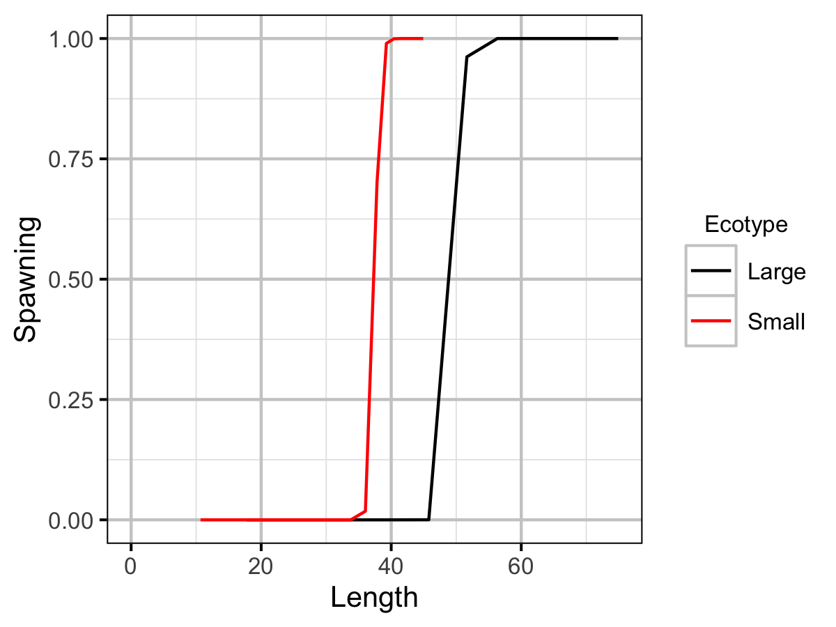
Ls	Large	5.00e+01	The length (or age if negative) at which 50 % mature (cm or yr).	Professional Judgement
Ls	Small	3.75e+01	The length (or age if negative) at which 50 % mature (cm or yr).	Spin Gillnetting
Sp	Small	1.00e+02	The maturity (as a function of length) power.	Default
es	Small	1.00e+00	The annual probability of a mature fish spawning.	Default
Sm	Small	0.00e+00	The spawning mortality probability.	Default
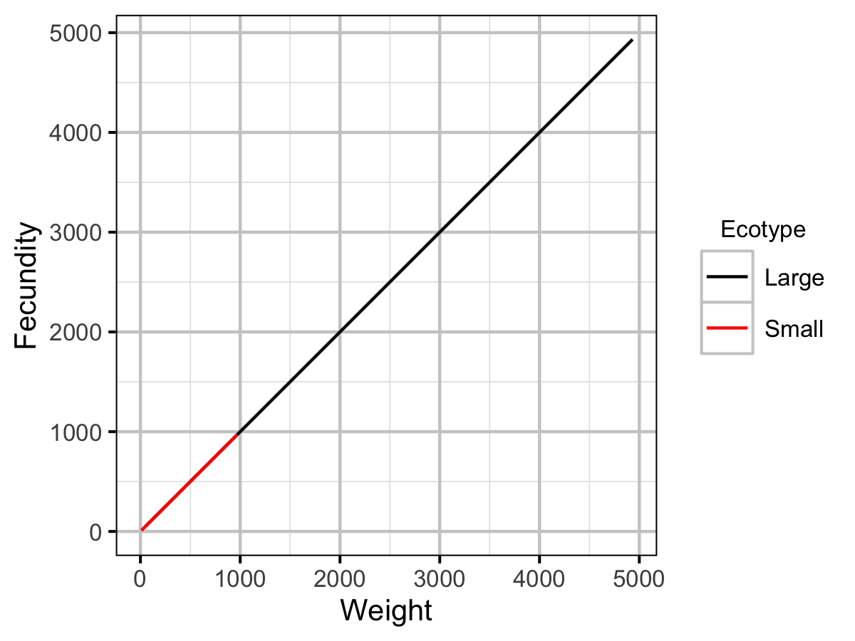
fb	Small	1.00e+00	The fecundity (as a function of weight) scaling exponent.	Default
tR	Small	1.00e+00	The age from which survival is density-independent (yr).	Default
BH	Small	1.00e+00	Recruitment follows a Beverton-Holt (1) or Ricker (0) relationship.	Default
Rk	Small	2.50e+01	The lifetime spawners per spawner at low density.	Myers et al. 1999
n	Small	1.50e-01	The annual interval natural mortality rate from age tR.	Default
nL	Small	1.09e-01	The annual interval natural mortality rate from length Ln.	Current Study
Ln	Small	5.00e+01	The length (or age if negative) at which the natural mortality rate switches from n to nL (cm or yr).	Default
Lv	Small	3.50e+01	The length (or age if negative) at which 50 % vulnerable to harvest (cm or yr).	Professional Judgement
Vp	Small	2.50e+01	The vulnerability to harvest (as a function of length) power.	Professional Judgement
Llo	Small	0.00e+00	The lower harvest slot length (cm).	Default
Lup	Small	1.00e+02	The upper harvest slot length (cm).	Default
Nc	Small	0.00e+00	The slot limits non-compliance probability.	Default
pi	Small	9.25e-02	The annual capture probability.	Current Study
rho	Small	0.00e+00	The release probability.	Default
Hm	Small	0.00e+00	The hooking mortality probability.	Default
Rmax	Small	1.00e+00	The number of recruits at the carrying capacity (ind).	Default
Wa	Small	5.37e-03	The (extrapolated) weight of a 1 cm individual (g).	Current Study
fa	Small	1.00e+00	The (theoretical) fecundity of a 1 g female (eggs).	Default
q	Small	1.00e-01	The catchability (annual probability of capture) for a unit of effort.	Default

Table 14. Lake Trout large ecotype yield-per-recruit calculations including the capture probability (pi), exploitation rate (u) and average age, length and weight of fish harvested.

Type	pi	u	Yield	Age	Length	Weight	Effort
actual	0.0924925	0.0924925	0.6246279	7.117998	55.04067	2142.810	0.9211561
optimal	0.1317662	0.1317662	0.6534407	6.369201	53.19010	1924.416	1.3410547

Table 15. Lake Trout small ecotype yield-per-recruit calculations including the capture probability (pi), exploitation rate (u) and average age, length and weight of fish harvested.

Type	pi	u	Yield	Age	Length	Weight	Effort
actual	0.0924925	0.0924925	0.0916155	10.260396	39.38564	652.8372	0.9211561
optimal	0.2924959	0.2924959	0.1305122	8.395765	37.74056	567.9933	3.2840757

Figures

Captures

figures/capture/CaptureMap.png — Figure 2. Lake Trout capture location by tagging.

figures/capture/CaptureRate.png — Figure 3. Capture rate by species and date for fish with fork length > 300 mm.

Coverage

figures/receiver/ReceiverMap.png — Figure 4. Location of sites with deployed receivers and estimated coverage (500m radius). Although receivers move slightly over time and after being redeployed, the centroid of all known locations for each receiver is shown.

Detections

figures/detection/DetectionOverview.png — Figure 5. Date of detections by species for each acoustically tagged fish. Grey segments indicate estimated tag life from capture date. Detections have been aggregated daily.

Condition

Growth

Survival

Yield-per-Recruit

figures/yield/AgeLength.png — Figure 10. Lake Trout assumed age by length and ecotype.

figures/yield/AgeWeight.png — Figure 11. Lake Trout assumed length by weight and ecotype.

figures/yield/LengthSpawning.png — Figure 12. Lake Trout assumed length by spawning and ecotype.

figures/yield/LengthVulnerability.png — Figure 13. Lake Trout assumed length by vulnerability to capture and ecotype.

figures/yield/WeightFecundity.png — Figure 14. Lake Trout assumed weight by fecundity and ecotype.

figures/yield/Yield.png — Figure 15. Lake Trout calculated yield as percent of total unfished biomass by annual interval fishing mortality rate and ecotype.

Recommendations

Recommendations include:

Continue annual mobile receiver surveys.

Acknowledgements

The organizations and individuals whose contributions have made this analytic appendix possible include:

MFLNRO - Cariboo Region
- Russ Bobrowski
- Scott Horley
Poisson Consulting Ltd.
- Evan Amies-Galonski

References

Bradford, Michael J, Josh Korman, and Paul S Higgins. 2005. “Using Confidence Intervals to Estimate the Response of Salmon Populations (Oncorhynchus Spp.) To Experimental Habitat Alterations.” Canadian Journal of Fisheries and Aquatic Sciences 62 (12): 2716–26. https://doi.org/10.1139/f05-179.

Brooks, Steve, Andrew Gelman, Galin L. Jones, and Xiao-Li Meng, eds. 2011. Handbook for Markov Chain Monte Carlo. Boca Raton: Taylor & Francis.

Fabrizio, Mary C., Bruce L. Swanson, Stephen T. Schram, and Michael H. Hoff. 1996. “Comparison of Three Nonlinear Models to Describe Long-Term Tag Shedding by Lake Trout.” Transactions of the American Fisheries Society 125 (2): 261–73. https://doi.org/10.1577/1548-8659(1996)125<0261:COTNMT>2.3.CO;2.

Gelman, Andrew, Daniel Simpson, and Michael Betancourt. 2017. “The Prior Can Often Only Be Understood in the Context of the Likelihood.” Entropy 19 (10): 555. https://doi.org/10.3390/e19100555.

Greenland, Sander. 2019. “Valid p -Values Behave Exactly as They Should: Some Misleading Criticisms of p -Values and Their Resolution With s -Values.” The American Statistician 73 (sup1): 106–14. https://doi.org/10.1080/00031305.2018.1529625.

Greenland, Sander, and Charles Poole. 2013. “Living with p Values: Resurrecting a Bayesian Perspective on Frequentist Statistics.” Epidemiology 24 (1): 62–68. https://doi.org/10.1097/EDE.0b013e3182785741.

He, Ji X., James R. Bence, James E. Johnson, David F. Clapp, and Mark P. Ebener. 2008. “Modeling Variation in Mass-Length Relations and Condition Indices of Lake Trout and Chinook Salmon in Lake Huron: A Hierarchical Bayesian Approach.” Transactions of the American Fisheries Society 137 (3): 801–17. https://doi.org/10.1577/T07-012.1.

Kery, Marc, and Michael Schaub. 2011. Bayesian Population Analysis Using WinBUGS : A Hierarchical Perspective. Boston: Academic Press. http://www.vogelwarte.ch/bpa.html.

McDermid, Jenni L., Brian J. Shuter, and Nigel P. Lester. 2010. “Life History Differences Parallel Environmental Differences Among North American Lake Trout (Salvelinus Namaycush) Populations.” Canadian Journal of Fisheries and Aquatic Sciences 67 (2): 314–25. https://doi.org/10.1139/F09-183.

Plummer, Martyn. 2015. “JAGS Version 4.0.1 User Manual.” http://sourceforge.net/projects/mcmc-jags/files/Manuals/4.x/.

R Core Team. 2020. “R: A Language and Environment for Statistical Computing.” Vienna, Austria: R Foundation for Statistical Computing. https://www.R-project.org/.

Thorley, Joseph L., and Greg F. Andrusak. 2017. “The Fishing and Natural Mortality of Large, Piscivorous Bull Trout and Rainbow Trout in Kootenay Lake, British Columbia (2008–2013).” PeerJ 5 (January): e2874. https://doi.org/10.7717/peerj.2874.

von Bertalanffy, L. 1938. “A Quantitative Theory of Organic Growth (Inquiries on Growth Laws Ii).” Human Biology 10: 181–213.

Walters, Carl J., and Steven J. D. Martell. 2004. Fisheries Ecology and Management. Princeton, N.J: Princeton University Press.