Kaslo Bull Trout Productivity 2019
The suggested citation for this analytic appendix is:
Thorley, J.L., Amies-Galonski, E. and Dalgarno, S.I.J. (2019) Kaslo Bull Trout Productivity 2019. A Poisson Consulting Analysis Appendix. URL: https://www.poissonconsulting.ca/f/168922378.
Background
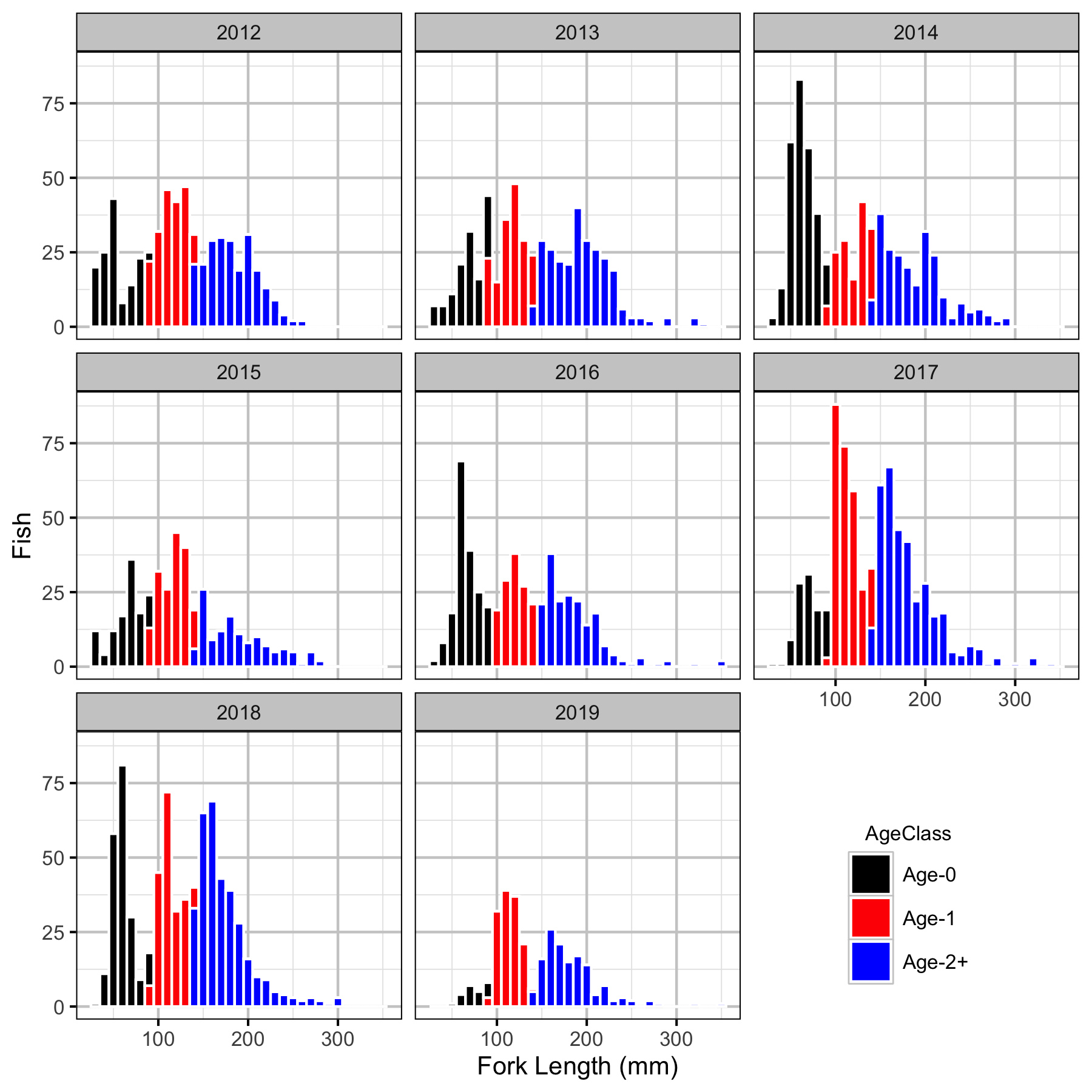
The Kaslo River and Keen Creek, which is a tributary of the Kaslo River, are important Bull Trout spawning and rearing tributaries on Kootenay Lake. From 2012 to 2019, field crews have night-snorkeled both systems in the fall and recorded all juvenile Bull Trout less than 350 mm in length. Snorkel and electrofishing marking crews have also captured and tagged juvenile Bull Trout for the snorkel crews to resight. Redd counts have been conducted in both systems since 2006.
The primary goal of the current analyses is to answer the following questions:
What is the observer efficiency when night-snorkeling for juvenile Bull Trout in the Kaslo River and Keen Creek?
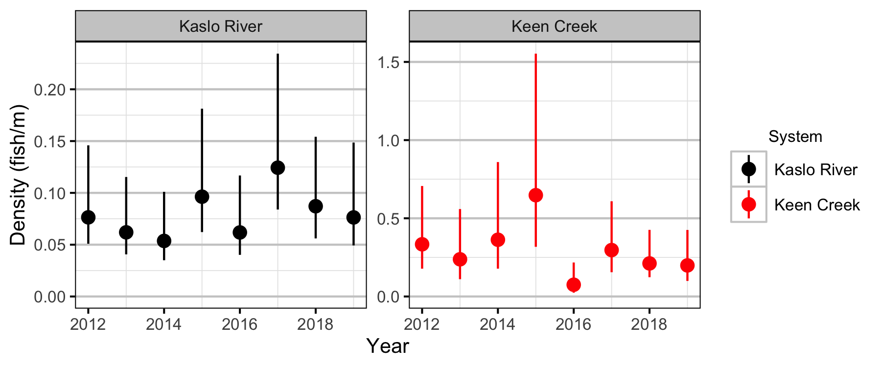
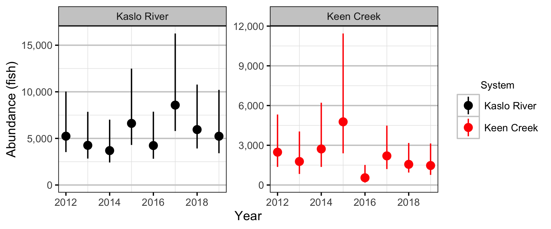
What are the densities of age-1 Bull Trout in the Kaslo River and Keen Creek?
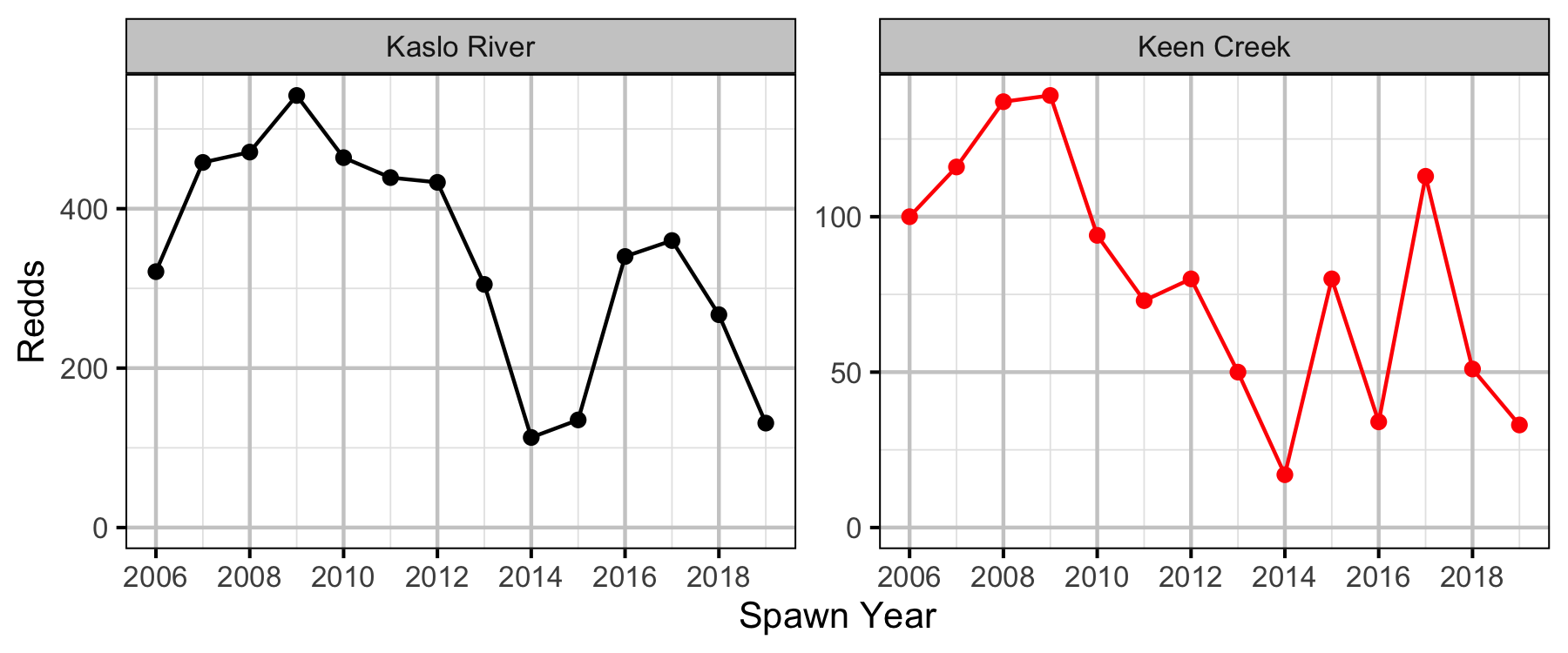
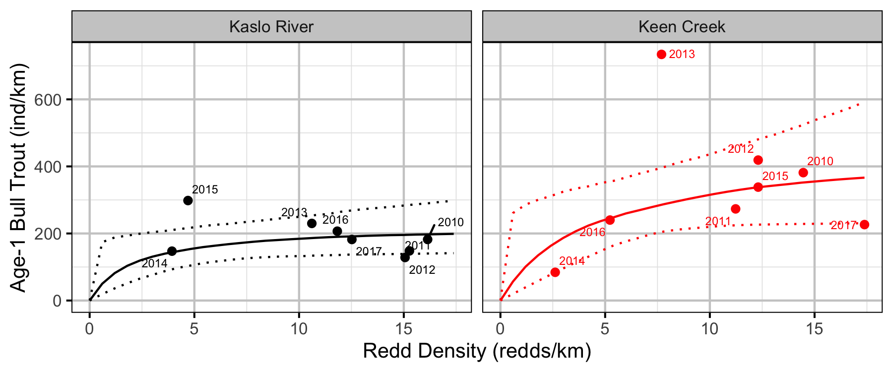
What is the relationship between the number of redds and the resultant densities of age-1 Bull Trout two years later?
Data Preparation
The data were cleaned, tidied and databased using R version 3.6.1 (R Core Team 2015).
Statistical Analysis
Model parameters were estimated using Maximum-Likelihood (ML) and Bayesian methods. The Maximum-Likelihood Estimates (MLE) were obtained using TMB (Kristensen et al. 2016) while the Bayesian estimates were produced using JAGS (Plummer 2015). For additional information on ML and Bayesian estimation the reader is referred to Millar (2011) and McElreath (2016), respectively.
Unless indicated otherwise, the Bayesian analyses used uninformative normal prior distributions (Kery and Schaub 2011, 36). The posterior distributions were estimated from 1500 Markov Chain Monte Carlo (MCMC) samples thinned from the second halves of 3 chains (Kery and Schaub 2011, 38–40). Model convergence was confirmed by ensuring that \(\hat{R} \leq 1.1\) (Kery and Schaub 2011, 40) and \(\textrm{ESS} \geq 150\) for each of the monitored parameters (Kery and Schaub 2011, 61). Where \(\hat{R}\) is the potential scale reduction factor and \(\textrm{ESS}\) is the effective sample size.
The parameters are summarised in terms of the point estimate, standard deviation (sd), the z-score, lower and upper 95% confidence/credible limits (CLs) and the p-value (Kery and Schaub 2011, 37, 42). For ML models, the point estimate is the MLE, the standard deviation is the standard error, the z-score is \(\mathrm{sd}/\mathrm{MLE}\) and the 95% CLs are the \(\mathrm{MLE} \pm 1.96 \cdot \mathrm{sd}\). For Bayesian models, the estimate is the median (50th percentile) of the MCMC samples, the z-score is \(\mathrm{sd}/\mathrm{mean}\) and the 95% CLs are the 2.5th and 97.5th percentiles. A p-value of 0.05 indicates that the lower or upper 95% CL is 0.
Model averaging and selection was implemented using an information theoretic approach (Burnham and Anderson 2002). ML models were compared using the marginal Akaike’s Information Criterion corrected for small sample size (AICc, Burnham and Anderson 2002). The support for fixed terms in models with identical random (Kery and Schaub 2011, 75) effects was assessed using the Akaike’s weights (\(w_i\)) (Burnham and Anderson 2002). The best supported model was then refitted as its Bayesian equivalent.
Where relevant, model adequacy was confirmed by examination of residual plots for the full model(s).
The results are displayed graphically by plotting the modeled relationships between particular variables and the response(s) with the remaining variables held constant. In general, continuous and discrete fixed variables are held constant at their mean and first level values, respectively, while random variables are held constant at their typical values (expected values of the underlying hyperdistributions) (Kery and Schaub 2011, 77–82). When informative the influence of particular variables is expressed in terms of the effect size (i.e., percent change in the response variable) with 95% confidence/credible intervals (CIs, Bradford, Korman, and Higgins 2005).
The analyses were implemented using R version 3.6.1
(R Core Team 2015) and the
mbr family of packages.
Model Descriptions
Length Correction
The annual bias (inaccuracy) and error (imprecision) in observer’s fish length estimates when spotlighting (standing) and snorkeling were quantified from the divergence of their length distribution from the length distribution for JLT and SH (the two most experience snorkelers) in that year. More specifically, the length correction that minimised the Jensen-Shannon divergence (Lin 1991) provided a measure of the inaccuracy while the minimum divergence (the Jensen-Shannon divergence was calculated with log to base 2 which means it lies between 0 and 1) provided a measure of the imprecision.
Observer Efficiency
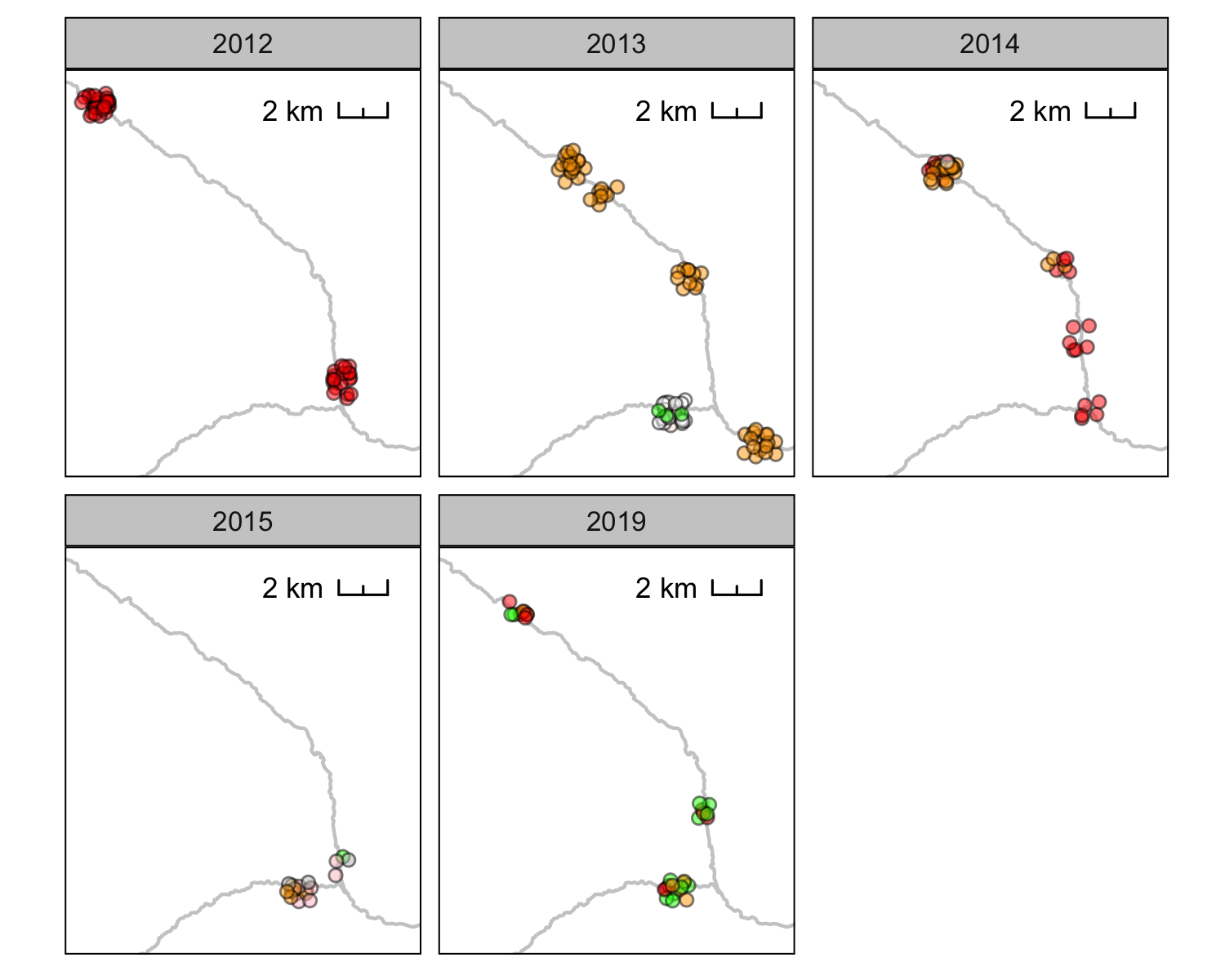
All resighted fish with a tag were allocated to the closest unallocated marked fish (with the same colour tag) by fork length and distance. The marked fish were analysed using a logistic regression model. Key assumptions of the full Maximum Likelihood logistic regression include:
- The observer efficiency varies by the fork length as a second order polynomial.
- The observer efficiency varies by observer.
- The observer efficiency varies between systems.
- The observer efficiency varies by the gradient, sinuosity and river kilometre.
Preliminary analysis indicated that river kilometre received similar support to watershed area.
The final Bayesian logistic regression assumed that:
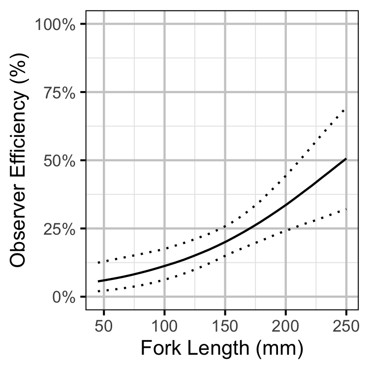
- The observer efficiency varies by the fork length.
Lineal Density
Both systems were broken into 100 m sites by bank. The lineal density at each site was estimated using an over-dispersed Poisson Generalized Linear Mixed Model. Key assumptions of the full Maximum Likelihood GLMM include:
- The lineal density varies between systems and years.
- The lineal density varies randomly by site.
- The lineal density varies by site sinuosity, gradient and river kilometre.
- The observer efficiency for each system is as estimated by the observer efficiency model.
Preliminary analysis indicated that river kilometre was better supported as a predictor of lineal density than watershed area. Preliminary analysis also indicated that autocorrelation (modeled as an AR1 process) was not significant.
The final Bayesian GLMM dropped sinuosity and gradient and took into account the uncertainty in the observer efficiencies as estimated by the observer efficiency model.
Stock-Recruitment
The stock-recruitment relationship was estimated using a Bayesian Beverton-Holt stock-recruitment curve. Key assumptions of the final BH SR model include:
- The strength of density-dependence varies between systems.
Model Templates
Observer Efficiency
Maximum Likelihood
.#include <TMB.hpp>

template<class Type>
Type objective_function<Type>::operator() () {
DATA_VECTOR(Observed);
DATA_FACTOR(Observer);
DATA_FACTOR(System);
DATA_VECTOR(Tagged);
DATA_VECTOR(Length);
DATA_VECTOR(Gradient);
DATA_VECTOR(Sinuosity);
DATA_VECTOR(Rkm);

PARAMETER(bSystem);
PARAMETER(bLength);
PARAMETER(bLength2);
PARAMETER(bGradient);
PARAMETER(bSinuosity);
PARAMETER(bRkm);

PARAMETER_VECTOR(bObserver);

vector<Type> eObserved = Observed;

int n = Observed.size();

Type nll = 0.0;

for(int i = 0; i < n; i++){
eObserved(i) = invlogit(bObserver(Observer(i)) + bSystem * System(i) + bLength * Length(i) + bLength2 * pow(Length(i), 2) + bGradient * Gradient(i) + bSinuosity * Sinuosity(i) + bRkm * Rkm(i));
nll -= dbinom(Observed(i), Tagged(i), eObserved(i), true);
return nll;
..
Block 1. Full model.
Bayesian
.model{
  bIntercept ~ dnorm(0, 5^-2)
  bLength ~ dnorm(0, 5^-2)

  for(i in 1:length(Observed)){
    logit(eObserved[i]) <-  bIntercept + bLength * Length[i]
    Observed[i] ~ dbern(eObserved[i])
  }
..
Block 2. Final model.
Lineal Density
Maximum Likelihood
.#include <TMB.hpp>

template<class Type>
Type objective_function<Type>::operator() () {
DATA_VECTOR(Count);
DATA_VECTOR(Length);
DATA_VECTOR(Coverage);
DATA_VECTOR(Efficiency);
DATA_VECTOR(Dispersion);

DATA_VECTOR(Gradient);
DATA_VECTOR(Sinuosity);
DATA_VECTOR(Rkm);

DATA_FACTOR(System);

DATA_FACTOR(Site);
DATA_INTEGER(nSite);
DATA_FACTOR(Year);

PARAMETER_MATRIX(bSystemYear);
PARAMETER_VECTOR(bSite);

PARAMETER(bGradient);
PARAMETER(bSinuosity);
PARAMETER(bRkm);

PARAMETER_VECTOR(bDispersion);
DATA_INTEGER(nDispersion);
PARAMETER(log_sDispersion);
PARAMETER(log_sSite);

Type sSite = exp(log_sSite);
Type sDispersion = exp(log_sDispersion);

ADREPORT(sSite);
ADREPORT(sDispersion);

vector<Type> eDensity = Count;
vector<Type> eCount = Count;
vector<Type> eNorm = pnorm(bDispersion, Type(0), Type(1));
vector<Type> eDispersion = qgamma(eNorm, pow(sDispersion, -2), pow(sDispersion, 2));

Type nll = 0.0;

for(int i = 0; i < nSite; i++){
nll -= dnorm(bSite(i), Type(0), sSite, true);

for(int i = 0; i < nDispersion; i++){
nll -= dnorm(bDispersion(i), Type(0), Type(1), true);

eDensity(i) = exp(bSystemYear(System(i), Year(i)) + bGradient * Gradient(i) + bSinuosity * Sinuosity(i) +  bRkm * Rkm(i) + bSite(Site(i)));
eCount(i) = eDensity(i) * Length(i) * Coverage(i);

nll -= dpois(Count(i), eCount(i) * Efficiency(i) * eDispersion(i), true);

return nll;
..
Block 3. The full model.
Bayesian
.model{

  bEfficiency ~ dnorm(Efficiency[1], EfficiencySD[1]^-2) T(0, )

  for(i in 1:nSystem) {
    for(j in 1:nYear) {
      bSystemYear[i,j] ~ dnorm(0, 5^-2)
    }
  }

  log_sSite ~ dnorm(0, 5^-2)
  log(sSite) <- log_sSite
  for(i in 1:nSite) {
    bSite[i] ~ dnorm(0, sSite^-2)
  }

  bRkm ~ dnorm(0, 5^-2)

  log_sDispersion ~ dnorm(0, 5^-2)
  log(sDispersion) <- log_sDispersion


  for(i in 1:length(Count)) {
    log(eDensity[i]) <- bSystemYear[System[i],Year[i]] + bRkm * Rkm[i] + bSite[Site[i]]
    eDispersion[i] ~ dgamma(sDispersion^-2, sDispersion^-2)
    Count[i] ~ dpois(eDensity[i] * Length[i] * Coverage[i] * bEfficiency * eDispersion[i])
  }
..
Block 4. The final model.
Stock-Recruiment
.model {
  log_bAlpha ~ dnorm(5, 5^-2)
  log(bAlpha) <- log_bAlpha

  for(i in 1:nSystem) {
    log_bBeta[i] ~ dnorm(0, 5^-2)
    log(bBeta[i]) <- log_bBeta[i]
  }

  log_sRecruits ~ dnorm(0, 5^-2)
  log(sRecruits) <- log_sRecruits

  for(i in 1:length(Recruits)){
    eRecruits[i] <- bAlpha * Stock[i] / (1 + bBeta[System[i]] * Stock[i])
    Recruits[i] ~ dlnorm(log(eRecruits[i]), sRecruits^-2)
  }
  bCarryingCapacity <- bAlpha / bBeta
..
Block 5. Final model.
Results
Tables
Coverage
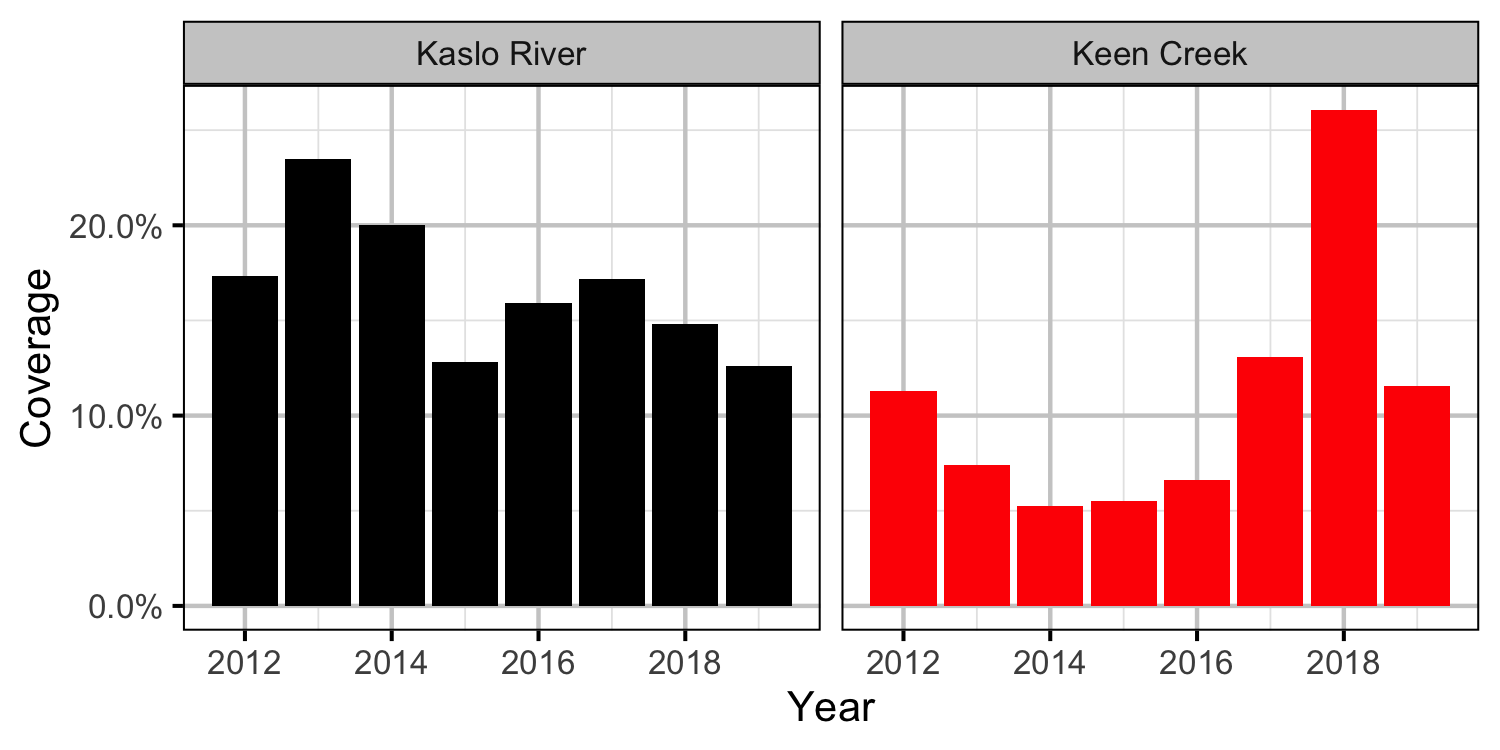
Table 1. Total length of river bank counted (including replicates) by system and year.
| System | Year | Length (km) |
|---|---|---|
| Kaslo River | 2012 | 10.57 [km] |
| Kaslo River | 2013 | 13.43 [km] |
| Kaslo River | 2014 | 11.45 [km] |
| Kaslo River | 2015 | 7.32 [km] |
| Kaslo River | 2016 | 11.59 [km] |
| Kaslo River | 2017 | 9.79 [km] |
| Kaslo River | 2018 | 8.43 [km] |
| Kaslo River | 2019 | 7.19 [km] |
| Keen Creek | 2012 | 1.44 [km] |
| Keen Creek | 2013 | 0.95 [km] |
| Keen Creek | 2014 | 0.67 [km] |
| Keen Creek | 2015 | 0.72 [km] |
| Keen Creek | 2016 | 0.85 [km] |
| Keen Creek | 2017 | 1.68 [km] |
| Keen Creek | 2018 | 3.37 [km] |
| Keen Creek | 2019 | 1.48 [km] |
Observer Efficiency
Table 2. Parameter descriptions.
| Parameter | Description |
|---|---|
bGradient |
The effect of Gradient on bIntercept |
bIntercept |
The intercept for logit(eObserved) |
bLength |
The effect of Length on bIntercept |
bLength2 |
The effect of Length on the effect of Length on bIntercept |
bRkm |
The effect of Rkm on bIntercept |
bSinuosity |
The effect of Sinuosity on bIntercept |
eObserved |
The expected probability of observing an individual |
Gradient |
The standardized site-level gradient |
Length |
The standardized fork length |
Observed |
The number of individuals observed (0 or 1) |
Rkm |
The standardized Rkm |
Sinuosity |
The standardized site-level sinuosity |
Tagged |
The number of tagged individuals (1) |
Maximum Likelihood
Table 3. Model averaged parameter estimates and Akaike weights.
| term | estimate | sd | zscore | lower | upper | pvalue | nmodels | proportion | ICWt |
|---|---|---|---|---|---|---|---|---|---|
| bGradient | 0.0918623 | 0.1509254 | 0.6086601 | -0.2039461 | 0.3876706 | 0.5427498 | 96 | 0.5000000 | 0.437 |
| bIntercept | -1.0808780 | 0.6371123 | -1.6965266 | -2.3295953 | 0.1678392 | 0.0897862 | 96 | 0.5000000 | 0.755 |
| bLength | 0.6677614 | 0.2038890 | 3.2751216 | 0.2681462 | 1.0673766 | 0.0010562 | 96 | 0.6666667 | 0.993 |
| bLength2 | -0.0425534 | 0.1231498 | -0.3455416 | -0.2839225 | 0.1988157 | 0.7296872 | 96 | 0.3333333 | 0.311 |
| bObserver[1] | -2.3082666 | 27.3607587 | -0.0843641 | -55.9343683 | 51.3178350 | 0.9327669 | 96 | 0.5000000 | 0.238 |
| bObserver[2] | -0.3257582 | 0.6112646 | -0.5329250 | -1.5238149 | 0.8722984 | 0.5940855 | 96 | 0.5000000 | 0.238 |
| bObserver[3] | -0.3072008 | 0.5629593 | -0.5456891 | -1.4105807 | 0.7961792 | 0.5852797 | 96 | 0.5000000 | 0.238 |
| bObserver[4] | -2.2142360 | 25.2858171 | -0.0875683 | -51.7735269 | 47.3450548 | 0.9302198 | 96 | 0.5000000 | 0.238 |
| bObserver[5] | -0.3711566 | 0.8717147 | -0.4257777 | -2.0796860 | 1.3373728 | 0.6702699 | 96 | 0.5000000 | 0.238 |
| bRkm | -0.0126214 | 0.1135448 | -0.1111581 | -0.2351652 | 0.2099224 | 0.9114910 | 96 | 0.5000000 | 0.268 |
| bSinuosity | -0.0094249 | 0.0883606 | -0.1066638 | -0.1826084 | 0.1637587 | 0.9150557 | 96 | 0.5000000 | 0.262 |
| bSystem | -0.0278483 | 0.2590061 | -0.1075198 | -0.5354908 | 0.4797943 | 0.9143766 | 96 | 0.5000000 | 0.269 |
Bayesian
Table 4. Final parameter estimates.
| term | estimate | sd | zscore | lower | upper | pvalue |
|---|---|---|---|---|---|---|
| bIntercept | -1.4809882 | 0.1929421 | -7.676471 | -1.8642345 | -1.138266 | 7e-04 |
| bLength | 0.6890303 | 0.2013763 | 3.464707 | 0.3319783 | 1.101899 | 7e-04 |
Table 5. Observer Efficiency estimates for a 123 mm Bull Trout.
| System | Efficiency | EfficiencySD | EfficiencyLower | EfficiencyUpper |
|---|---|---|---|---|
| Kaslo River | 0.1474655 | 0.0292574 | 0.0960496 | 0.207584 |
Table 6. Final model summary.
| n | K | nchains | niters | nthin | ess | rhat | converged |
|---|---|---|---|---|---|---|---|
| 220 | 2 | 3 | 500 | 1 | 573 | 1.005 | TRUE |
Lineal Density
Table 7. Parameter descriptions.
| Parameter | Description |
|---|---|
bDispersion |
The random effect of overdispersion |
bGradient |
The effect of Gradient on bSystemYear |
bRkm |
The effect of Rkm on bSystemYear |
bSinuosity |
The effect of Sinuosity on bSystemYear |
bSite |
The random effect of Site on bSystemYear |
bSystemYear |
The effect of System and Year on log(eDensity) |
Count |
Number of fish counted |
Coverage |
Proportion of site surveyed |
Dispersion |
Factor for random effect of overdispersion |
eCount |
The expected Count |
eDensity |
The expected lineal density |
Efficiency |
The observer efficiency from the observer efficiency model |
Gradient |
Standardized gradient |
Length |
Length of site (m) |
log_sDispersion |
log(sDispersion) |
log_sSite |
log(sSite) |
Rkm |
Standardized Rkm |
sDispersion |
The SD of bDispersion |
Sinuosity |
Standardized sinuosity |
Site |
The site |
sSite |
The SD of bSite |
System |
The system |
Year |
The year |
Maximum Likelihood
Table 8. Model averaged parameter estimates and Akaike weights.
| term | estimate | sd | zscore | lower | upper | pvalue | nmodels | proportion | ICWt |
|---|---|---|---|---|---|---|---|---|---|
| bGradient | 0.0311395 | 0.0454417 | 0.6852622 | -0.0579247 | 0.1202037 | 0.4931785 | 8 | 0.5 | 0.482 |
| bRkm | 0.4715056 | 0.0547874 | 8.6060899 | 0.3641242 | 0.5788871 | 0.0000000 | 8 | 0.5 | 0.999 |
| bSinuosity | 0.0363242 | 0.0456070 | 0.7964614 | -0.0530639 | 0.1257123 | 0.4257639 | 8 | 0.5 | 0.545 |
| bSystemYear[1,1] | -2.6455437 | 0.1121992 | -23.5789813 | -2.8654502 | -2.4256373 | 0.0000000 | 8 | 1.0 | 0.999 |
| bSystemYear[2,1] | -1.2172578 | 0.2447367 | -4.9737450 | -1.6969329 | -0.7375827 | 0.0000007 | 8 | 1.0 | 0.999 |
| bSystemYear[1,2] | -2.8589534 | 0.1051397 | -27.1919385 | -3.0650235 | -2.6528833 | 0.0000000 | 8 | 1.0 | 0.999 |
| bSystemYear[2,2] | -1.5767460 | 0.3377544 | -4.6683203 | -2.2387325 | -0.9147594 | 0.0000030 | 8 | 1.0 | 0.999 |
| bSystemYear[1,3] | -2.9864266 | 0.1161414 | -25.7137179 | -3.2140595 | -2.7587937 | 0.0000000 | 8 | 1.0 | 0.999 |
| bSystemYear[2,3] | -1.1402911 | 0.3443506 | -3.3114251 | -1.8152058 | -0.4653764 | 0.0009282 | 8 | 1.0 | 0.999 |
| bSystemYear[1,4] | -2.4212448 | 0.1254062 | -19.3072247 | -2.6670364 | -2.1754533 | 0.0000000 | 8 | 1.0 | 0.999 |
| bSystemYear[2,4] | -0.5882569 | 0.3099003 | -1.8982133 | -1.1956504 | 0.0191365 | 0.0576680 | 8 | 1.0 | 0.999 |
| bSystemYear[1,5] | -2.8513065 | 0.1148164 | -24.8336078 | -3.0763426 | -2.6262704 | 0.0000000 | 8 | 1.0 | 0.999 |
| bSystemYear[2,5] | -2.7100919 | 0.5109829 | -5.3036836 | -3.7116000 | -1.7085837 | 0.0000001 | 8 | 1.0 | 0.999 |
| bSystemYear[1,6] | -2.1502622 | 0.0983227 | -21.8694488 | -2.3429711 | -1.9575533 | 0.0000000 | 8 | 1.0 | 0.999 |
| bSystemYear[2,6] | -1.3561990 | 0.2486467 | -5.4543206 | -1.8435377 | -0.8688604 | 0.0000000 | 8 | 1.0 | 0.999 |
| bSystemYear[1,7] | -2.5353756 | 0.1163632 | -21.7884632 | -2.7634433 | -2.3073079 | 0.0000000 | 8 | 1.0 | 0.999 |
| bSystemYear[2,7] | -1.6811798 | 0.2023087 | -8.3099714 | -2.0776976 | -1.2846620 | 0.0000000 | 8 | 1.0 | 0.999 |
| bSystemYear[1,8] | -2.6358901 | 0.1298255 | -20.3033252 | -2.8903434 | -2.3814367 | 0.0000000 | 8 | 1.0 | 0.999 |
| bSystemYear[2,8] | -1.7410385 | 0.2792599 | -6.2344738 | -2.2883778 | -1.1936992 | 0.0000000 | 8 | 1.0 | 0.999 |
| log_sDispersion | -0.6849019 | 0.1069518 | -6.4038346 | -0.8945236 | -0.4752801 | 0.0000000 | 8 | 1.0 | 0.999 |
| log_sSite | -0.8235911 | 0.1355269 | -6.0769561 | -1.0892190 | -0.5579633 | 0.0000000 | 8 | 1.0 | 0.999 |
Bayesian
Table 9. Parameter estimates.
| term | estimate | sd | zscore | lower | upper | pvalue |
|---|---|---|---|---|---|---|
| bEfficiency | 0.1378714 | 0.0298430 | 4.580539 | 0.0741621 | 0.1939628 | 0.0007 |
| bRkm | 0.4783569 | 0.0556769 | 8.568303 | 0.3671965 | 0.5855429 | 0.0007 |
| bSystemYear[1,1] | -2.5719482 | 0.2662244 | -9.535631 | -2.9771583 | -1.9249779 | 0.0007 |
| bSystemYear[2,1] | -1.0970516 | 0.3484160 | -3.097938 | -1.7267405 | -0.3472264 | 0.0080 |
| bSystemYear[1,2] | -2.7818108 | 0.2597451 | -10.617058 | -3.2019452 | -2.1599471 | 0.0007 |
| bSystemYear[2,2] | -1.4362010 | 0.4259282 | -3.330629 | -2.2011092 | -0.5812363 | 0.0053 |
| bSystemYear[1,3] | -2.9255387 | 0.2684283 | -10.783027 | -3.3525650 | -2.2922316 | 0.0007 |
| bSystemYear[2,3] | -1.0137786 | 0.4060204 | -2.416645 | -1.7259986 | -0.1512328 | 0.0227 |
| bSystemYear[1,4] | -2.3400137 | 0.2682543 | -8.619585 | -2.7778505 | -1.7078437 | 0.0007 |
| bSystemYear[2,4] | -0.4341576 | 0.4031108 | -1.034867 | -1.1468397 | 0.4401022 | 0.2907 |
| bSystemYear[1,5] | -2.7836306 | 0.2688845 | -10.241027 | -3.2140260 | -2.1472869 | 0.0007 |
| bSystemYear[2,5] | -2.5888360 | 0.5501223 | -4.725784 | -3.7170614 | -1.5263210 | 0.0007 |
| bSystemYear[1,6] | -2.0849773 | 0.2552975 | -8.040223 | -2.4775737 | -1.4508127 | 0.0007 |
| bSystemYear[2,6] | -1.2145196 | 0.3426224 | -3.516282 | -1.8631924 | -0.4959314 | 0.0027 |
| bSystemYear[1,7] | -2.4405574 | 0.2646835 | -9.155318 | -2.8815792 | -1.8697727 | 0.0007 |
| bSystemYear[2,7] | -1.5533202 | 0.3127407 | -4.912500 | -2.0925553 | -0.8532112 | 0.0007 |
| bSystemYear[1,8] | -2.5728975 | 0.2777654 | -9.151591 | -3.0097806 | -1.9068394 | 0.0007 |
| bSystemYear[2,8] | -1.6155660 | 0.3686062 | -4.362258 | -2.3086733 | -0.8543728 | 0.0007 |
| log_sDispersion | -0.6079784 | 0.1030649 | -5.957853 | -0.8318048 | -0.4140571 | 0.0007 |
| log_sSite | -0.8346942 | 0.1538637 | -5.510836 | -1.1895857 | -0.6001209 | 0.0007 |
Table 10. Model summary.
| n | K | nchains | niters | nthin | ess | rhat | converged |
|---|---|---|---|---|---|---|---|
| 982 | 20 | 3 | 500 | 20 | 134 | 1.019 | FALSE |
Stock-Recruiment
Table 11. Parameter descriptions.
| Parameter | Description |
|---|---|
bBeta |
Density-dependence |
eRecruits |
Expected value of Recruits |
Recruits |
Number of age-1 Bull Trout |
Stock |
Number of Bull Trout redds |
bAlpha |
Recruits per stock at low stock density |
sRecruits |
SD of residual variation in Recruits |
Bayesian
Table 12. Final parameter estimates.
| term | estimate | sd | zscore | lower | upper | pvalue |
|---|---|---|---|---|---|---|
| bAlpha | 107.9617072 | 6.959718e+03 | 0.1256190 | 33.5430430 | 3998.2911962 | 0.0007 |
| bBeta[1] | 0.4966219 | 3.690286e+01 | 0.1224021 | 0.0769660 | 23.7598897 | 0.0007 |
| bBeta[2] | 0.2378008 | 2.501060e+01 | 0.1184190 | 0.0030618 | 13.2126752 | 0.0007 |
| bCarryingCapacity[1] | 224.2683120 | 9.128826e+02 | 0.2946850 | 149.2815777 | 488.7363168 | 0.0007 |
| bCarryingCapacity[2] | 456.6886954 | 6.821273e+05 | 0.0336592 | 244.7990487 | 11760.8229020 | 0.0007 |
| log_bAlpha | 4.6817766 | 1.210229e+00 | 4.1163117 | 3.5128293 | 8.2933643 | 0.0007 |
| log_bBeta[1] | -0.6999266 | 1.388835e+00 | -0.3402677 | -2.5644317 | 3.1679938 | 0.5347 |
| log_bBeta[2] | -1.4363280 | 1.932357e+00 | -0.7136175 | -5.7887633 | 2.5811351 | 0.3373 |
| log_sRecruits | -0.8019392 | 2.074041e-01 | -3.7961545 | -1.1573710 | -0.3456840 | 0.0007 |
| sRecruits | 0.4484585 | 1.005801e-01 | 4.6247301 | 0.3143116 | 0.7077362 | 0.0007 |
Table 13. Final model summary.
| n | K | nchains | niters | nthin | ess | rhat | converged |
|---|---|---|---|---|---|---|---|
| 16 | 10 | 3 | 500 | 100 | 288 | 1.012 | TRUE |
Figures
Systems
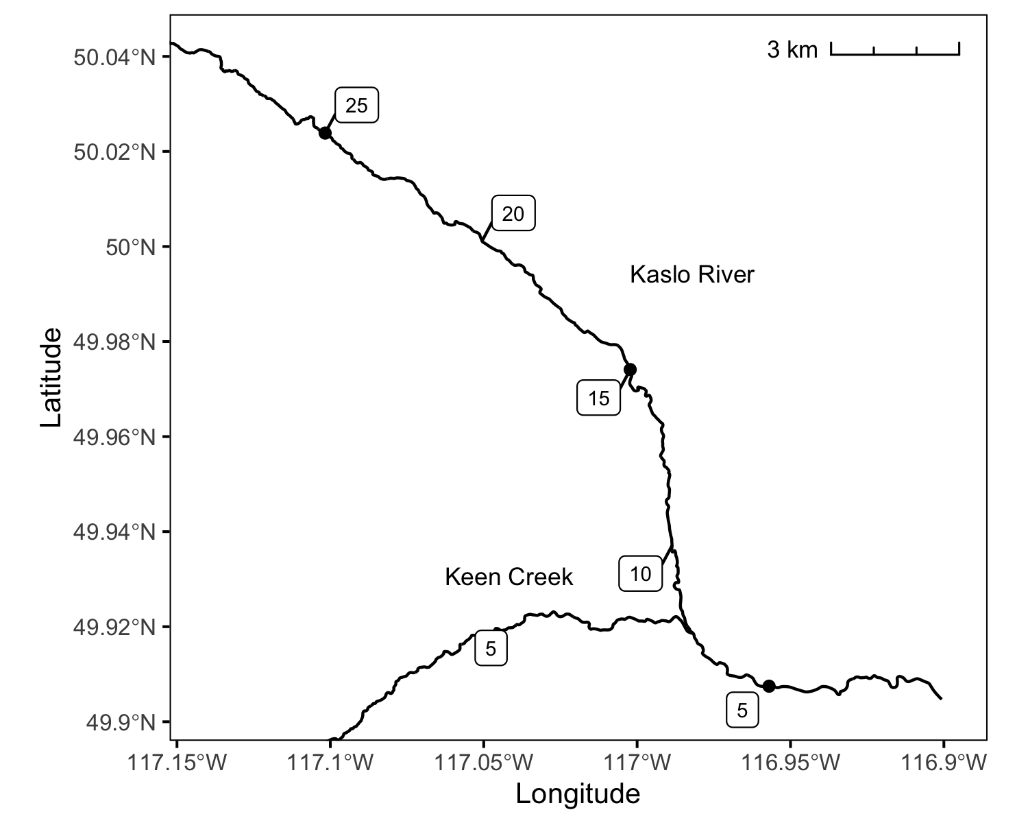
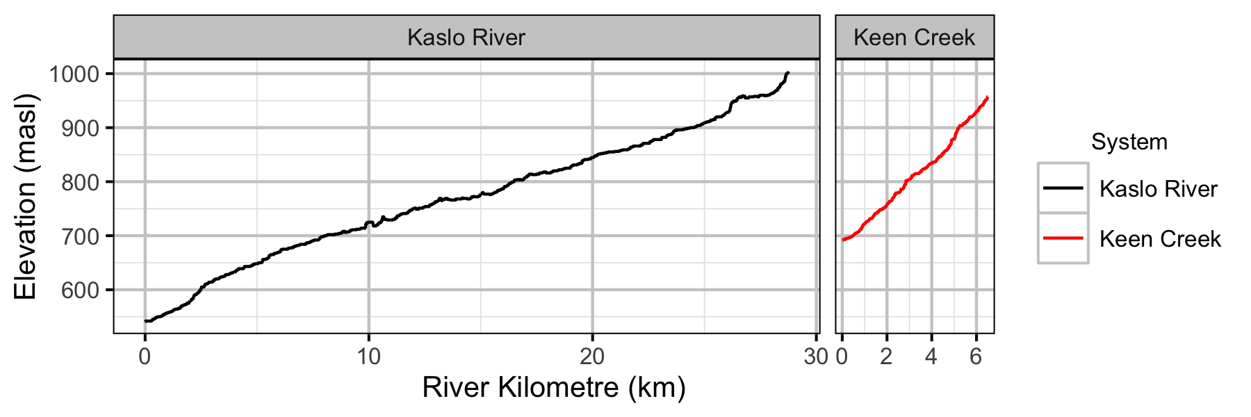
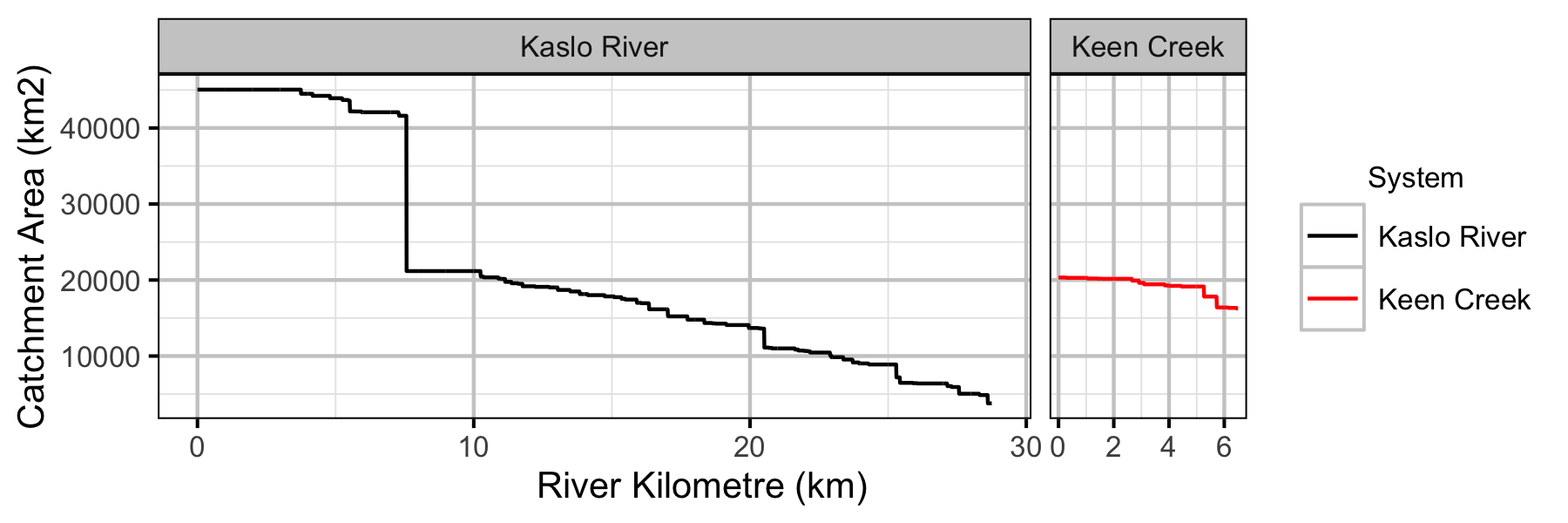
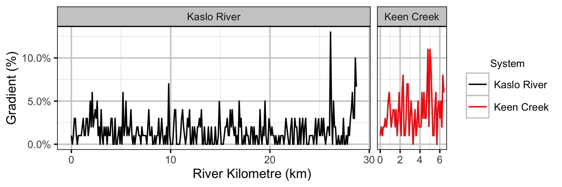
Sites
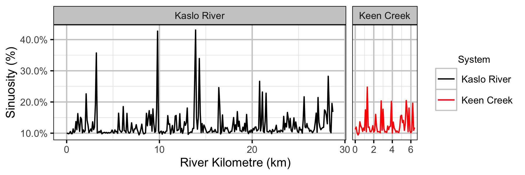
Coverage
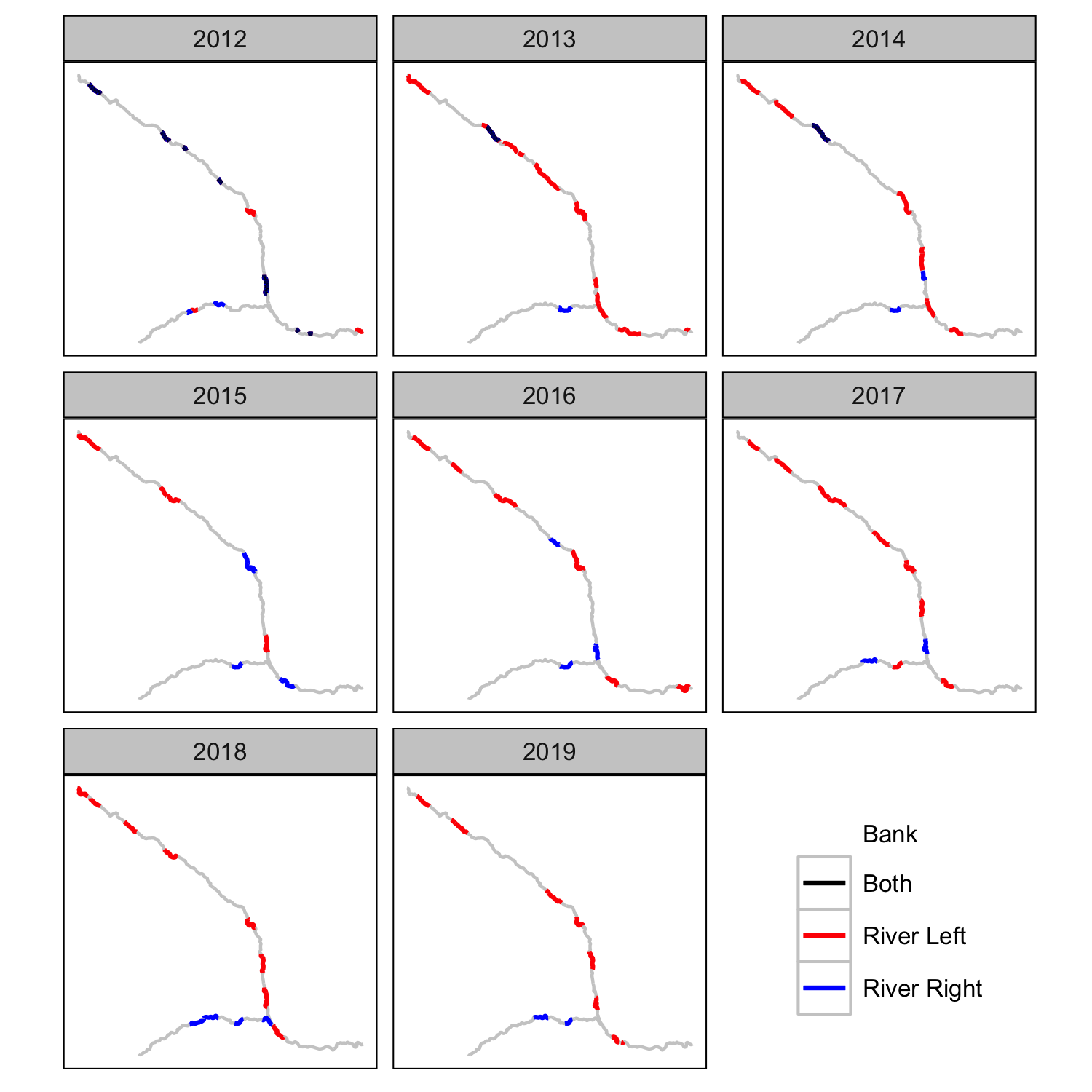
Length Correction
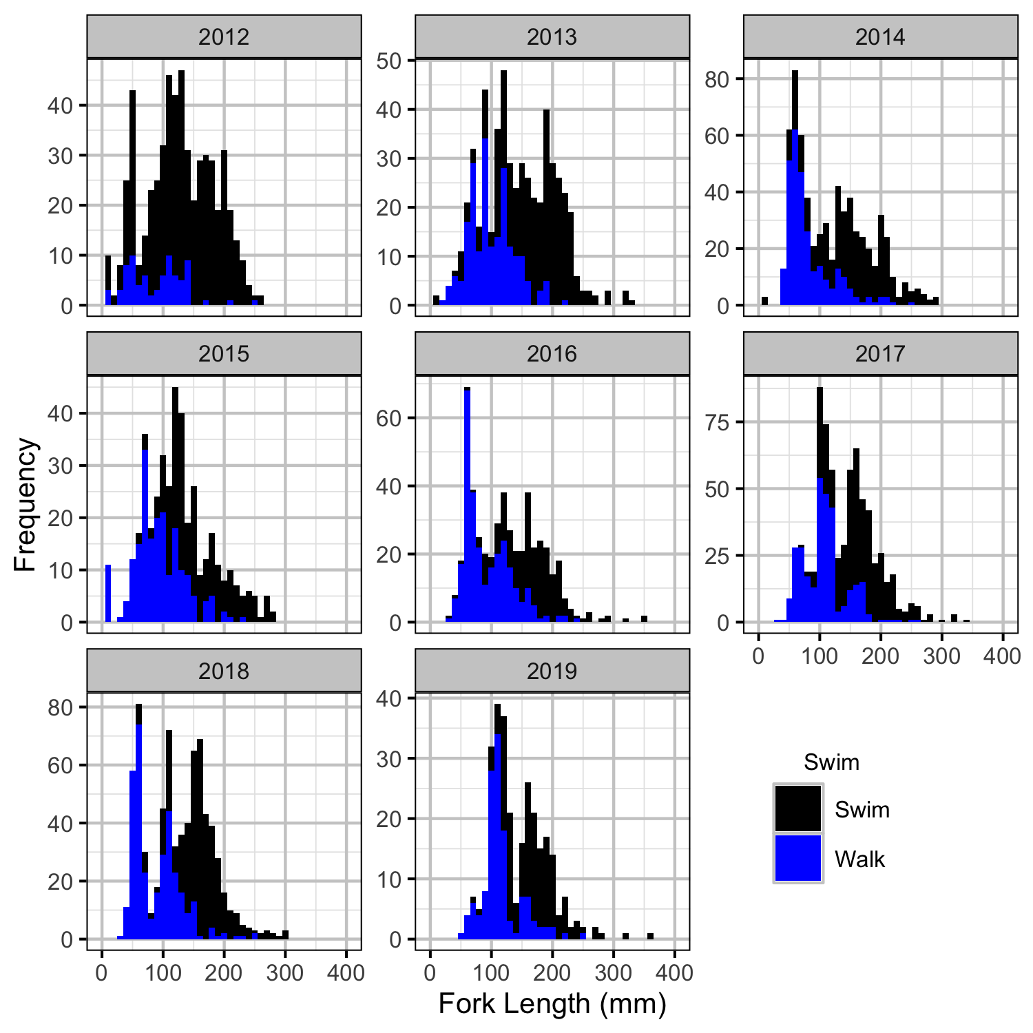
Fish
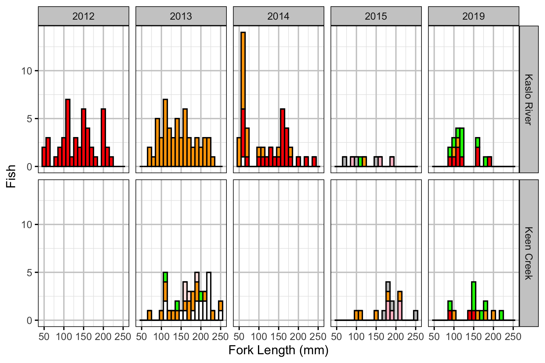
Observer Efficiency
Bayesian
Lineal Density
Stock-Recruiment
Conclusions
- Observer efficiency is approximately 17% for age-1 Bull Trout.
- Age-1 Bull Trout are relatively evenly distributed with respect to mesohabitat.
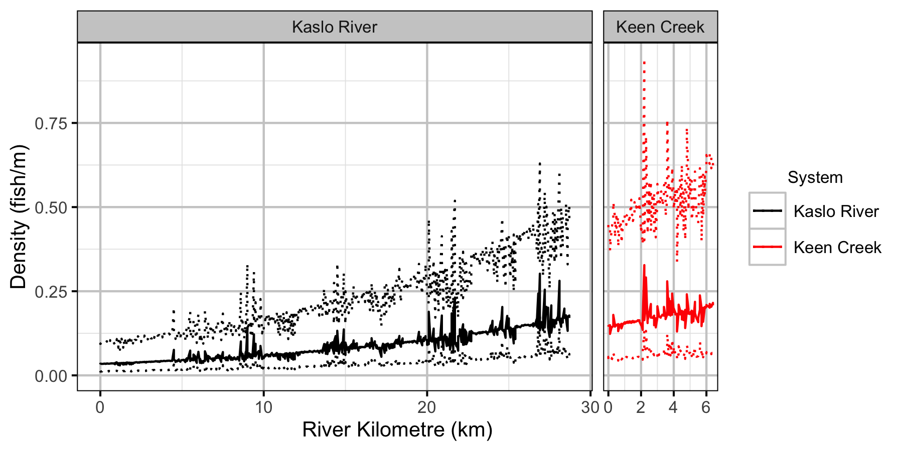
- Lineal densities of age-1 Bull Trout increase with river kilometre in both systems.
- The age-1 carrying capacity is estimated to be around 220 fish per km in Kaslo River and around 440 fish per km in Keen Creek.
Acknowledgements
The organisations and individuals whose contributions have made this analysis report possible include:
- Habitat Conservation Trust Foundation
- Ministry of Forest, Lands and Natural Resource Operations
- Greg Andrusak
- Ministry of Environment
- Jen Sarchuk
- BC Fish and Wildlife
- Trina Radford
- Stephan Himmer
- Gillian Sanders
- Jeff Berdusco
- Vicky Lipinski
- Jimmy Robbins
- Jason Bowers
References
Bradford, Michael J, Josh Korman, and Paul S Higgins. 2005. “Using Confidence Intervals to Estimate the Response of Salmon Populations (Oncorhynchus Spp.) to Experimental Habitat Alterations.” Canadian Journal of Fisheries and Aquatic Sciences 62 (12): 2716–26. https://doi.org/10.1139/f05-179.
Burnham, Kenneth P., and David R. Anderson. 2002. Model Selection and Multimodel Inference: A Practical Information-Theoretic Approach. Vol. Second Edition. New York: Springer.
Kery, Marc, and Michael Schaub. 2011. Bayesian Population Analysis Using WinBUGS : A Hierarchical Perspective. Boston: Academic Press. http://www.vogelwarte.ch/bpa.html.
Kristensen, Kasper, Anders Nielsen, Casper W. Berg, Hans Skaug, and Bradley M. Bell. 2016. “TMB : Automatic Differentiation and Laplace Approximation.” Journal of Statistical Software 70 (5). https://doi.org/10.18637/jss.v070.i05.
Lin, J. 1991. “Divergence Measures Based on the Shannon Entropy.” IEEE Transactions on Information Theory 37 (1): 145–51. https://doi.org/10.1109/18.61115.
McElreath, Richard. 2016. Statistical Rethinking: A Bayesian Course with Examples in R and Stan. Chapman & Hall/CRC Texts in Statistical Science Series 122. Boca Raton: CRC Press/Taylor & Francis Group.
Millar, R. B. 2011. Maximum Likelihood Estimation and Inference: With Examples in R, SAS, and ADMB. Statistics in Practice. Chichester, West Sussex: Wiley.
Plummer, Martyn. 2015. “JAGS Version 4.0.1 User Manual.” http://sourceforge.net/projects/mcmc-jags/files/Manuals/4.x/.
R Core Team. 2015. “R: A Language and Environment for Statistical Computing.” Vienna, Austria: R Foundation for Statistical Computing. http://www.R-project.org/.