Kootenay Lake Exploitation Study 2013
The suggested citation for this analytic report is:
Thorley, J.L. (2014) Kootenay Lake Exploitation Study 2013. A Poisson Consulting Analysis Report. URL: https://www.poissonconsulting.ca/f/1088509848.
Background
The Kootenay Lake Exploitation Study is a multi-year fish tagging program to estimate the proportion of large rainbow and bull trout that are caught by anglers versus die of natural causes on Kootenay Lake.
Methods
Data
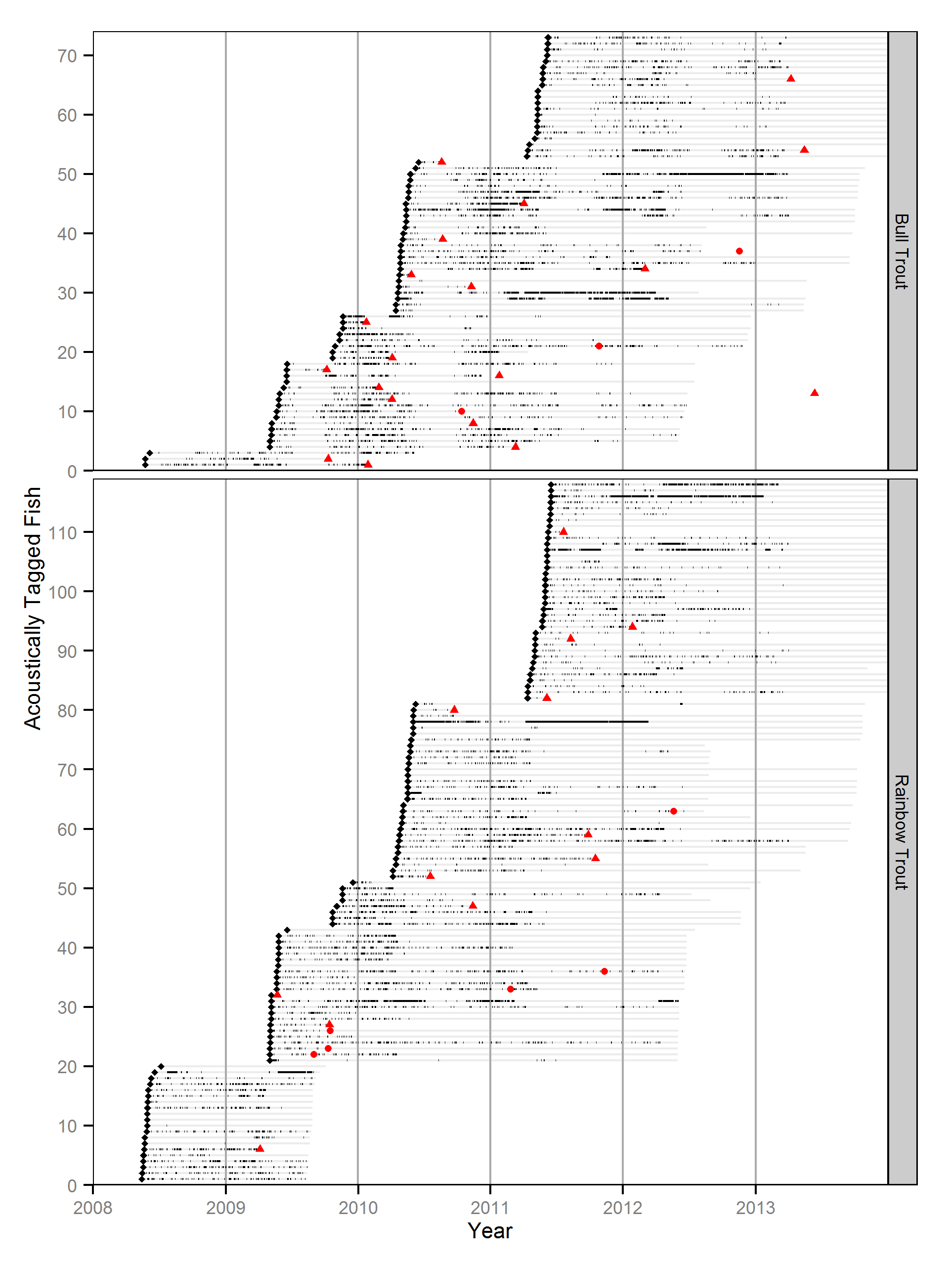
The data were collected by releasing large (\(\ge\) 500 mm) rod caught rainbow trout and bull trout with acoustic tags and T-bar reward tags. An acoustic receiver array detected movements of the fish while anglers reported recaptures.
| Species | Year | Tagged | 2009 | 2010 | 2011 | 2012 | 2013 |
|---|---|---|---|---|---|---|---|
| Bull Trout | 2008 | 3 | 1 | 1 | 0 | 0 | 0 |
| Bull Trout | 2009 | 23 | 1 | 6 | 3 | 0 | 1 |
| Bull Trout | 2010 | 26 | 0 | 4 | 1 | 2 | 0 |
| Bull Trout | 2011 | 21 | 0 | 0 | 0 | 0 | 2 |
| Rainbow Trout | 2008 | 20 | 1 | 0 | 0 | 0 | 0 |
| Rainbow Trout | 2009 | 31 | 5 | 1 | 2 | 0 | 0 |
| Rainbow Trout | 2010 | 30 | 0 | 2 | 2 | 1 | 0 |
| Rainbow Trout | 2011 | 37 | 0 | 0 | 3 | 1 | 0 |
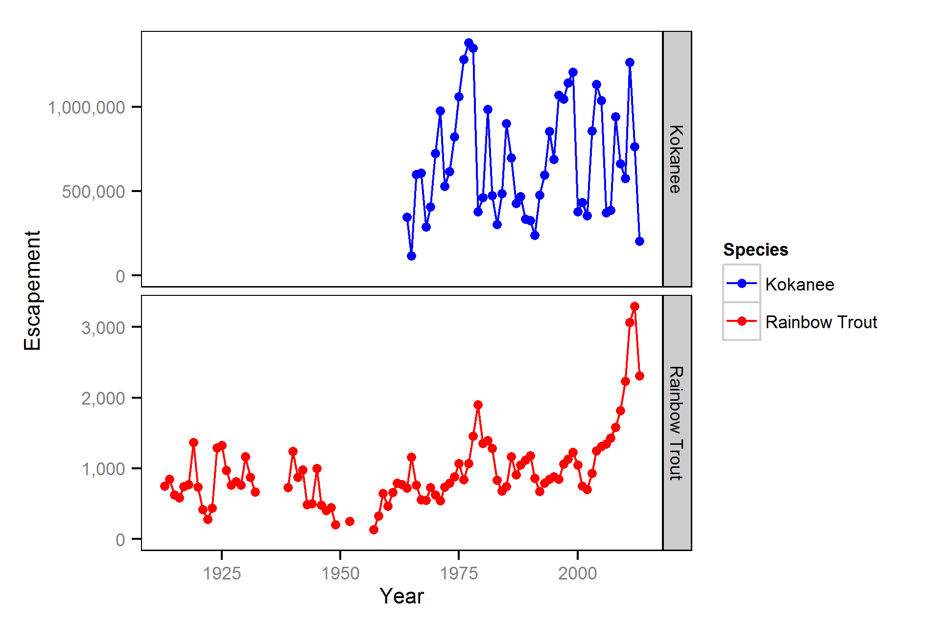
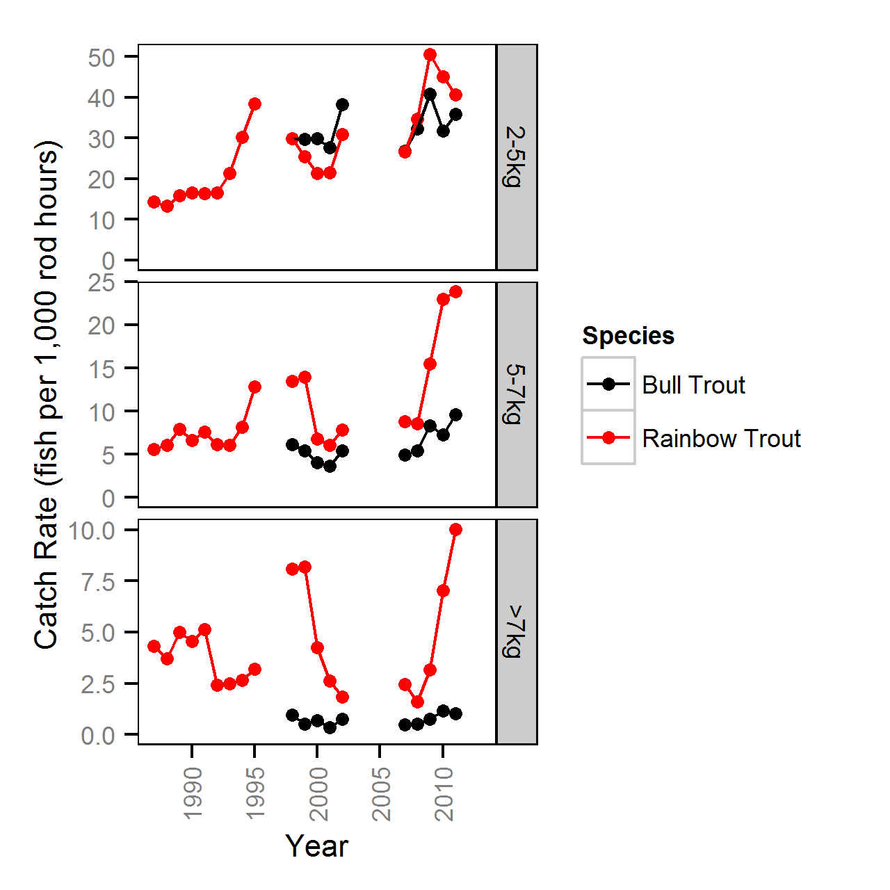
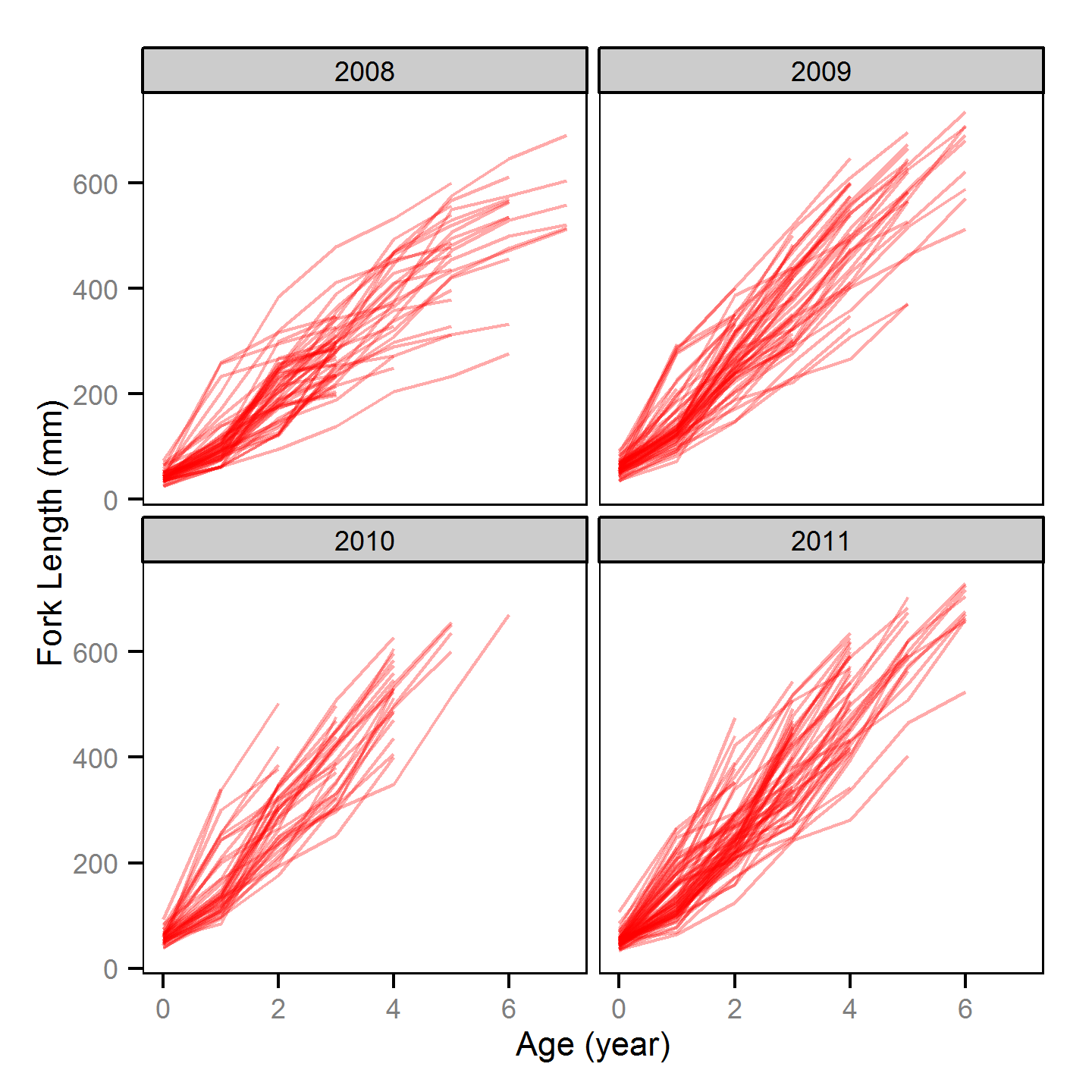
The back-calculation of length-at-age from scale samples was conducted by Greg Andrusak of Redfish Consulting Ltd. The Ministry of Forests, Lands and Natural Resource Operations (MFLNRO) provided spawner escapement estimates for kokanee in Meadow Creek spawning channel and rainbow trout at Gerrard as well as data from the Kootenay Lake Rainbow Trout (KLRT) mailout survey.
Statistical Analysis
Hierarchical Bayesian models were fitted to the rainbow and bull trout tagging, acoustic detection and angler return data for Kootenay Lake using R version 3.0.3 (Team, 2013) and JAGS 3.3.0 (Plummer, 2012) which interfaced with each other via jaggernaut 1.7 (Thorley, 2014). For additional information on hierarchical Bayesian modelling in the BUGS language, of which JAGS uses a dialect, the reader is referred to Kery and Schaub (2011) pages 41-44.
Unless specified, the models assumed vague (low information) prior distributions (Kéry and Schaub, 2011, p. 36). The posterior distributions were estimated from a minimum of 1,000 Markov Chain Monte Carlo (MCMC) samples thinned from the second halves of three chains (Kéry and Schaub, 2011, pp. 38-40). Model convergence was confirmed by ensuring that Rhat (Kéry and Schaub, 2011, p. 40) was less than 1.1 for each of the parameters in the model (Kéry and Schaub, 2011, p. 61). When possible model adequacy was confirmed by examination of residual plots.
The posterior distributions of the fixed (Kéry and Schaub, 2011, p. 75) parameters are summarised below in terms of a point estimate (mean), lower and upper 95% credible limits (2.5th and 97.5th percentiles), the standard deviation (SD), percent relative error (half the 95% credible interval as a percent of the point estimate) and significance (Kéry and Schaub, 2011, p. 37,42).
When none of the candidate models included random effects, model selection was achieved by choosing the model with the lower Deviance Information Criterion (DIC) value. Otherwise model selection was achieved by percent relative error-based backwards stepwise variable selection (Kéry and Schaub, 2011, p. 42) from the full model until all the variables had a percent relative error less than 100. This is approximately equivalent to dropping insignificant (p > 0.05) fixed variables and uninformative random (Kéry and Schaub, 2011, pp. 77-82) variables.
The results are displayed graphically by plotting the modeled relationships between particular variables and the response with 95% credible intervals (CRIs) with the remaining variables held constant. In general, continuous and discrete fixed variables are held constant at their mean and first level values respectively while random variables are held constant at their typical values (expected values of the underlying hyperdistributions) (Kéry and Schaub, 2011, pp. 77-82). Where informative the influence of particular variables is expressed in terms of the effect size (i.e., percent change in the response variable) with 95% credible intervals (Bradford et al. 2005). Through the report bull trout data and estimates are plotted in black while rainbow trout are plotted in red. Plots were produced using the ggplot2 R package (Wickham, 2009).
Body Condition
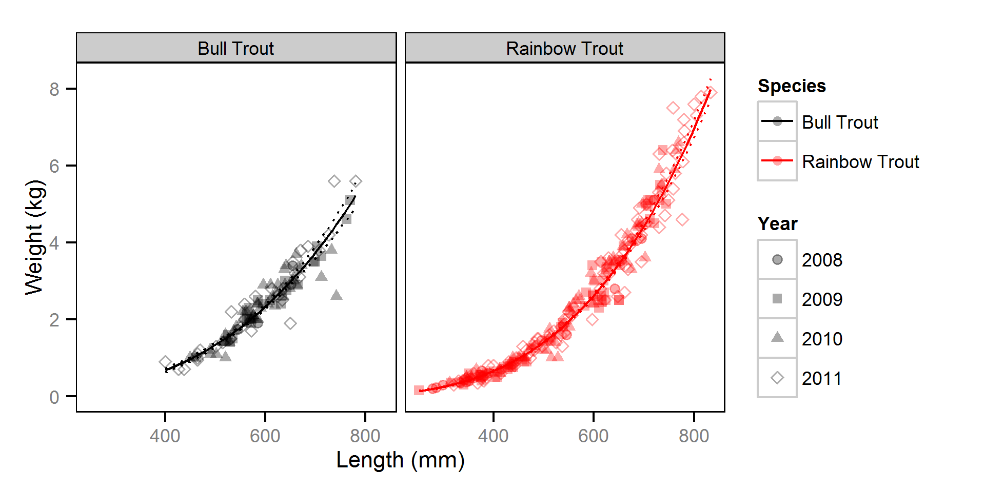
Temporal variation in condition (body weight when accounting for body length) was estimated from the initial captures using a mass-length model (He et al. 2008).
Key assumptions of the full condition model include:
- Weight varies with fork length and day of the year (as a second order polynomial).
- Weight varies randomly with year.
- The residual variation in weight is log-normally distributed.
Competing models were fitted without year and/or day of the year.
Short-Term Hooking Mortality
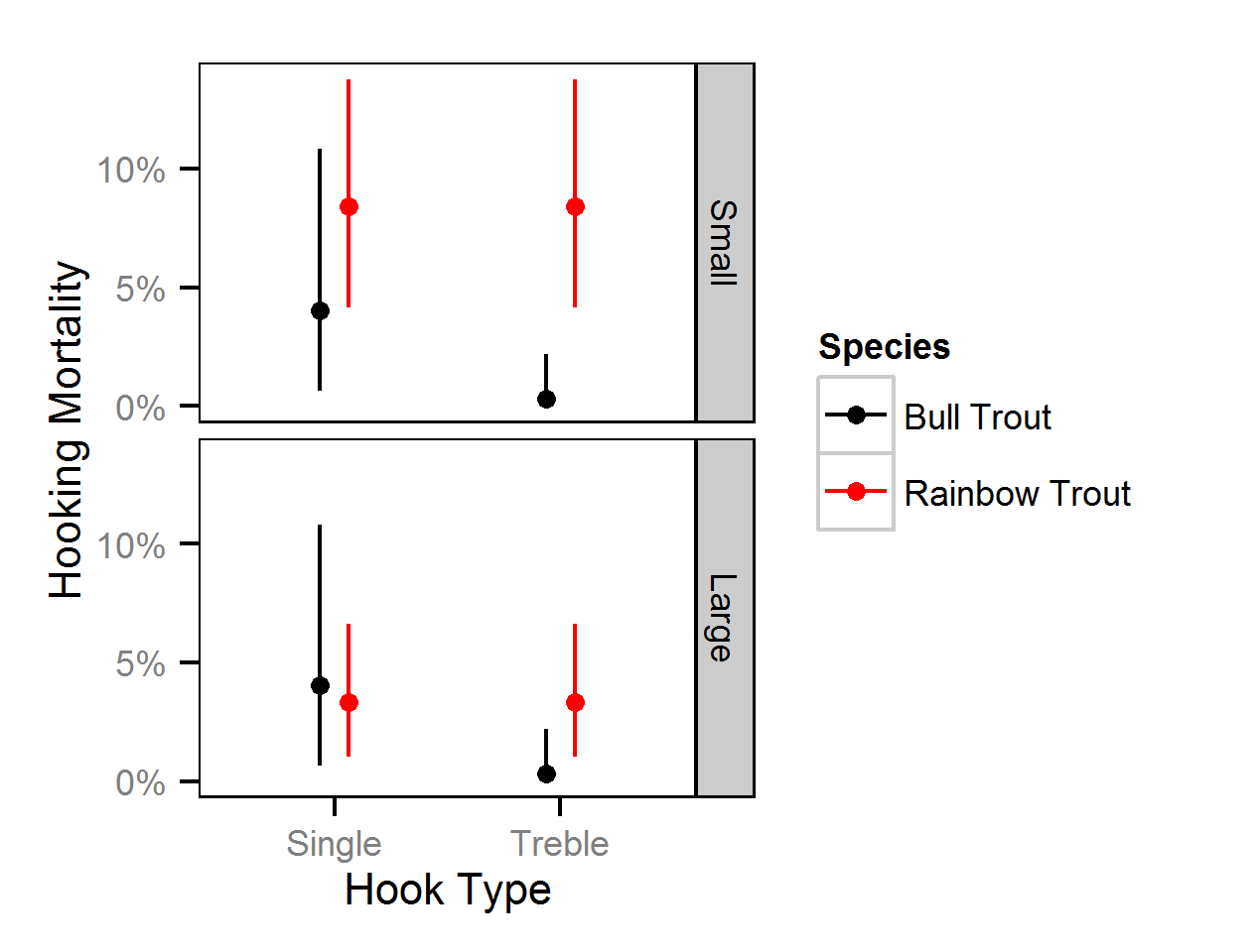
Short-term (pre-release) hooking mortality was estimated from the initial captures using a two-way ANOVA (Kéry and Schaub, 2011, pp. 100-106) with an interaction and a binomial (logistic) response.
Key assumptions of the hooking mortality model include:
- Hooking mortality varies with fish size (small versus large) and hook type (single versus treble) and the interaction between the two.
- Observed hooking mortality is Bernoulli distributed.
Competing models were fitted without the fish size and/or hook type effects and their interaction.
T-bar Tag Loss
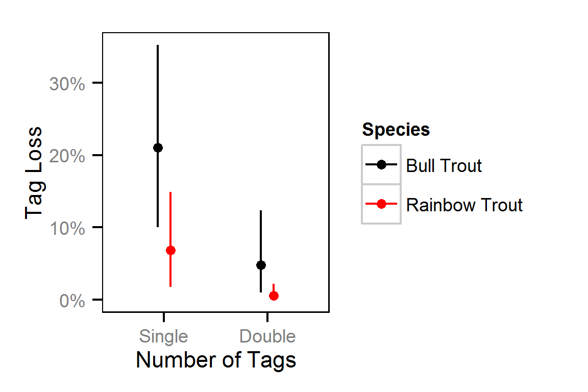
T-bar tag loss was estimated from the number of tags reported from recaught double-tagged individuals (Fabrizio et al. 1999).
Key assumptions of the tag loss model include:
- The probability of tag loss is independent between tags on a fish.
- Reported tag numbers are described by a zero-truncated binomial distribution (as fish that had lost both tags were not reportable).
Preliminary analyses indicated that there were insufficient recaptures to include days at large or fish length as explanatory variables.
Harvest Rates
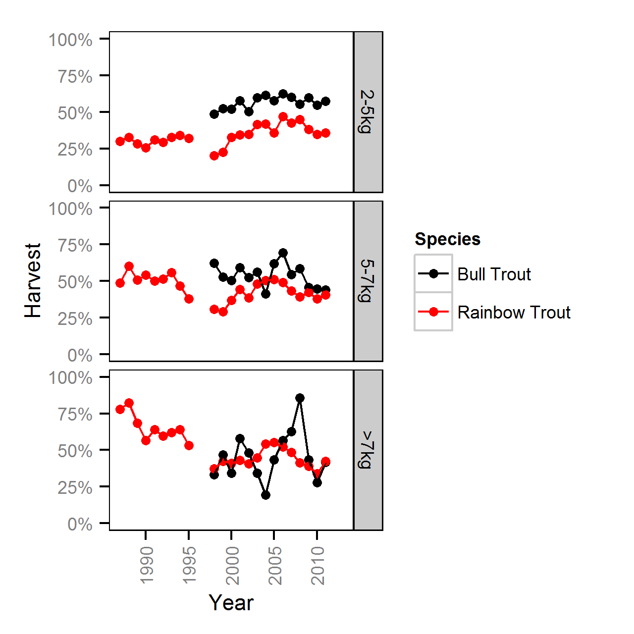
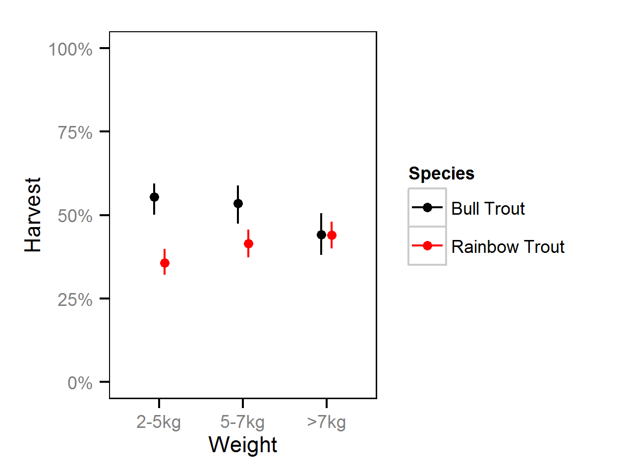
Harvest rates were estimated from the number of fish reported caught and harvested in the KLRT mailout survey since 1999 using a logistic ANOVA.
Key assumptions of the full harvest model include:
- The harvest rate varies with weight class (2-5, 5-7 and >7kg).
- The number of fish harvested is described by an overdispersed binomial distribution.
Competing models were fitted without the weight effect.
Annual Growth
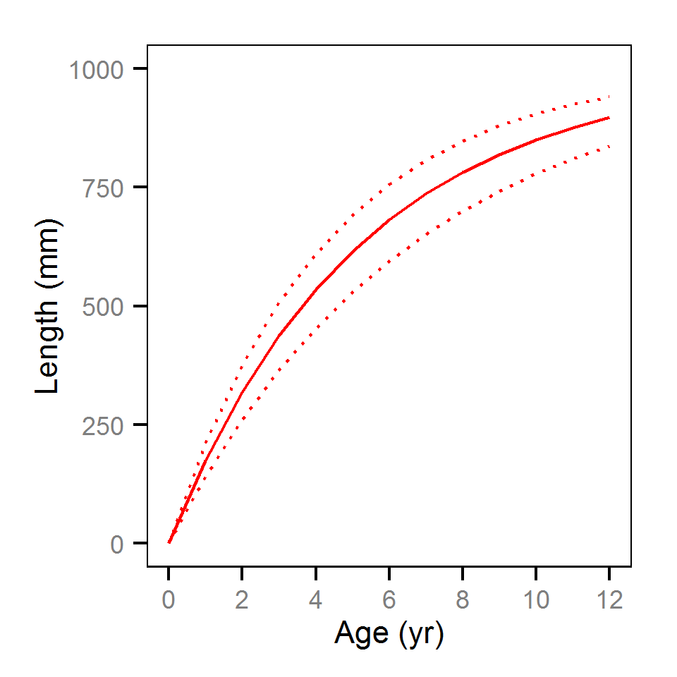
Annual growth was estimated from the initial capture’s scale-based back-calculated lengths using the Fabens form of the Von Bertalanffy growth model (He and Bence, 2007).
Key assumptions of the full growth model include:
- Annual length increments from age 3 and older are described by a Von Bertalanffy growth curve.
- The length-at-infinity is 1000 mm.
- Time at length 0 is 0.
- The growth coefficient (k) varies randomly with year and fish.
- Residual annual length increments are normally distributed.
Competing models were fitted without the annual and/or individual variation in k.
Natural and Fishing Mortality
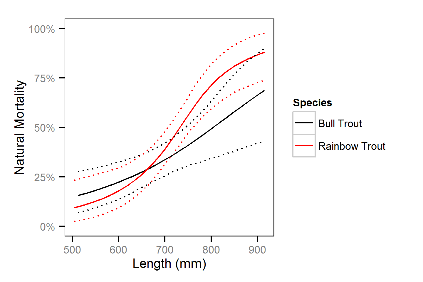
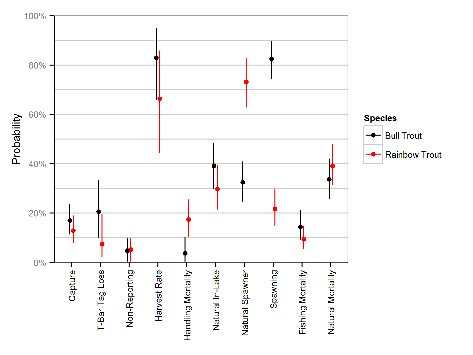
Natural and fishing mortality was estimated from the acoustic detection and tag reporting data using a Cormack-Jolly-Seber state-space model (Kéry and Schaub, 2011, pp. 175-177).
Key assumptions of the mortality model include:
- One year consists of four discrete time intervals (seasons) of 3 months.
- Log-odds probability of the loss of a T-bar tag is normally distributed with a mean of -1.37 and a SD of 0.40 for bull trout and a mean of -2.75 and SD of 0.57 for rainbow trout as estimated by the T-bar Tag Loss models.
- Non-reporting of T-bar tagged angled fish uniformly ranges between 0 and 10%.
- Change in length is as described by a Von Bertalanffy growth curve with a length-at-infinity of 1000 mm and a growth coefficient (k) of 0.19.
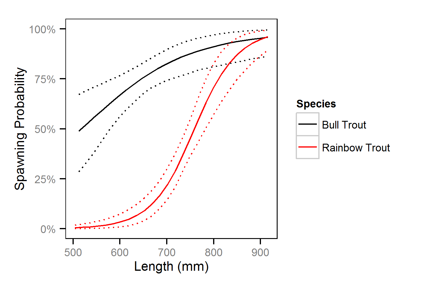
- Probability of spawning is independent of whether a fish spawned in the previous year.
- Probability of spawning varies with length.
- Probability of capture by an angler varies randomly with year.
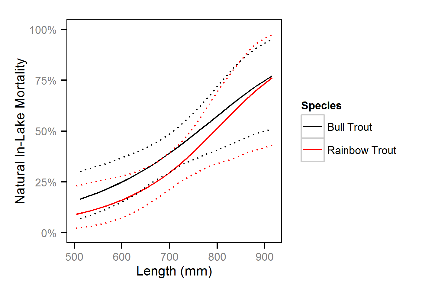
- Natural mortality differs between in-lake versus spawners.
- In-lake natural mortality varies with length.
Preliminary analyses indicated that length and season were not significant predictors and year was not an informative predictor of capture probability.
Model Code
The JAGS model code, which uses a series of naming conventions, is presented below.
Body Condition
| Variable/Parameter | Description |
|---|---|
bWeight |
Intercept for log(eWeight) |
bWeightDayte |
Effect of standardized day of the year on log(eWeight) |
bWeightDayte2 |
Quadratic effect of standardized day of the year on log(eWeight) |
bWeightLength |
Effect of centered log length on log(eWeight) |
bWeightYear[i] |
Effect of ith year on log(eWeight) |
Dayte[i] |
Standardised day of year on which the ith fish was caught |
eWeight[i] |
Expected weight of ith fish |
Length[i] |
Centered log length of ith fish |
sWeight |
SD of log-normally distributed residual weight |
Weight[i] |
Weight of ith fish |
Body Condition - Model1
model {

  bWeight ~ dnorm(0, 2^-2)
  bWeightLength ~ dnorm(3, 2^-2)
  bWeightDayte ~ dnorm(0, 2^-2)
  bWeightDayte2 ~ dnorm(0, 2^-2)

  sWeightYear ~ dunif(0, 2)
  for (i in 1:nYear) {
    bWeightYear[i] ~ dnorm(0, sWeightYear^-2)
  }

  sWeight ~ dunif(0, 2)

  for(i in 1:length(Length)) {

    log(eWeight[i]) <- bWeight
        + bWeightLength * Length[i]
        + bWeightDayte * Dayte[i]
        + bWeightDayte2 * Dayte[i]^2
        + bWeightYear[Year[i]]

    Weight[i] ~ dlnorm(log(eWeight[i]), sWeight^-2)
  }
}
Body Condition - Model2
model {

  bWeight ~ dnorm(0, 2^-2)
  bWeightLength ~ dnorm(3, 2^-2)

  sWeightYear ~ dunif(0, 2)
  for (i in 1:nYear) {
    bWeightYear[i] ~ dnorm(0, sWeightYear^-2)
  }

  sWeight ~ dunif(0, 2)

  for(i in 1:length(Length)) {

    log(eWeight[i]) <- bWeight
      + bWeightLength * Length[i]
      + bWeightYear[Year[i]]

    Weight[i] ~ dlnorm(log(eWeight[i]), sWeight^-2)
  }
}
Body Condition - Model3
model {

  bWeight ~ dnorm(0, 2^-2)
  bWeightLength ~ dnorm(3, 2^-2)
  bWeightDayte ~ dnorm(0, 2^-2)
  bWeightDayte2 ~ dnorm(0, 2^-2)

  sWeight ~ dunif(0, 2)

  for(i in 1:length(Length)) {

    log(eWeight[i]) <- bWeight
      + bWeightLength * Length[i]
      + bWeightDayte * Dayte[i]
      + bWeightDayte2 * Dayte[i]^2

    Weight[i] ~ dlnorm(log(eWeight[i]), sWeight^-2)
  }
}
Body Condition - Model4
model {

  bWeight ~ dnorm(0, 2^-2)
  bWeightLength ~ dnorm(3, 2^-2)

  sWeight ~ dunif(0, 2)

  for(i in 1:length(Length)) {

    log(eWeight[i]) <- bWeight
      + bWeightLength * Length[i]

    Weight[i] ~ dlnorm(log(eWeight[i]), sWeight^-2)
  }
}
Short-Term Hooking Mortality
| Variable/Parameter | Description |
|---|---|
bMortality |
Intercept for logit(eMortality[i]) |
bMortalityHookType[i] |
Effect of ith hook type on logit(eMortality[i]) |
bMortalitySize[i] |
Effect of ith fish size on logit(eMortality[i]) |
bMortalitySizeHookType[i, j] |
Effect of interaction between ith fish size and jth hook type on logit(eMortality[i]) |
eMortality[i] |
Predicted probability of a hooking mortality for ith fish |
Mortality[i] |
Observed hooking mortality of ith fish |
Short-Term Hooking Mortality - Model1
model{

  bMortality ~ dnorm(0, 5^-2)

  bMortalitySize[1] <- 0
  for (i in 2:nSize) {
    bMortalitySize[i] ~ dnorm(0, 5^-2)
  }

  bMortalityHookType[1] <- 0
  for (i in 2:nHookType) {
    bMortalityHookType[i] ~ dnorm(0, 5^-2)
  }

  for (j in 1:nHookType) {
    bMortalitySizeHookType[1, j] <- 0
  }

  for (i in 2:nSize) {
      bMortalitySizeHookType[i, 1] <- 0
      for (j in 2:nHookType) {
          bMortalitySizeHookType[i, j] ~ dnorm(0, 5^-2)
      }
  }

  for(i in 1:length(Mortality)) {

    logit(eMortality[i]) <- bMortality
      + bMortalitySize[Size[i]]
      + bMortalityHookType[HookType[i]]
      + bMortalitySizeHookType[Size[i], HookType[i]]

    Mortality[i] ~ dbern(eMortality[i])
  }
}
Short-Term Hooking Mortality - Model2
model{

  bMortality ~ dnorm(0, 5^-2)

  bMortalitySize[1] <- 0
  for (i in 2:nSize) {
    bMortalitySize[i] ~ dnorm(0, 5^-2)
  }

  bMortalityHookType[1] <- 0
  for (i in 2:nHookType) {
    bMortalityHookType[i] ~ dnorm(0, 5^-2)
  }

  for(i in 1:length(Mortality)) {

    logit(eMortality[i]) <- bMortality
      + bMortalitySize[Size[i]]
      + bMortalityHookType[HookType[i]]

    Mortality[i] ~ dbern(eMortality[i])
  }
}
Short-Term Hooking Mortality - Model3
model{

  bMortality ~ dnorm(0, 5^-2)

  bMortalitySize[1] <- 0
  for (i in 2:nSize) {
    bMortalitySize[i] ~ dnorm(0, 5^-2)
  }

  for(i in 1:length(Mortality)) {

  logit(eMortality[i]) <- bMortality
    + bMortalitySize[Size[i]]

  Mortality[i] ~ dbern(eMortality[i])
  }
}
Short-Term Hooking Mortality - Model4
model{

  bMortality ~ dnorm(0, 5^-2)

  bMortalityHookType[1] <- 0
  for (i in 2:nHookType) {
    bMortalityHookType[i] ~ dnorm(0, 5^-2)
  }

  for(i in 1:length(Mortality)) {

    logit(eMortality[i]) <- bMortality
      + bMortalityHookType[HookType[i]]

    Mortality[i] ~ dbern(eMortality[i])
  }
}
Short-Term Hooking Mortality - Model5
model{

  bMortality ~ dnorm(0, 5^-2)

  for(i in 1:length(Mortality)) {

  logit(eMortality[i]) <- bMortality

  Mortality[i] ~ dbern(eMortality[i])
  }
}
T-Bar Tag Loss
| Variable/Parameter | Description |
|---|---|
| bTagLossIntercept | Intercept for logit(eTagLoss) |
| eTagLoss[i] | Predicted probability of single tag loss for ith recapture |
| TagsRecap[i] | Tags remaining on ith recapture |
T-Bar Tag Loss - Model1
model{
  bTagLossIntercept ~ dnorm(0, 2^-2)

  for (i in 1:length(TagsRecap)) {
    logit(eTagLoss[i]) <- bTagLossIntercept

    TagsRecap[i] ~ dbin(1 - eTagLoss[i], 2) T(1, )
  }
}
Harvest Rates
| Variable/Parameter | Description |
|---|---|
bHarvest |
Intercept for logit(eHarvest) |
bHarvestWeight[i] |
Effect of ith weight class on logit(eHarvest) |
Catch[i] |
Number of fish in ith year-weight class caught |
eHarvest[i] |
Predicted harvest rate for ith year-weight class |
Harvest[i] |
Number of fish in ith year-weight class harvested |
Harvest Rates - Model1
model{

  bHarvest ~ dnorm(0, 2^-2)

  bHarvestWeight[1] <- 0
  for(i in 2:nWeight) {
    bHarvestWeight[i] ~ dnorm(0, 2^-2)
  }

  sDispersion ~ dunif(0, 2)
  for(i in 1:length(Harvest)) {

    eDispersion[i] ~ dnorm(0, sDispersion^-2)

    logit(eHarvest[i]) <- bHarvest
      + bHarvestWeight[Weight[i]]
      + eDispersion[i]

    Harvest[i] ~ dbin(eHarvest[i], Catch[i])
  }
}
Harvest Rates - Model2
model{

  bHarvest ~ dnorm(0, 2^-2)

  sDispersion ~ dunif(0, 2)
  for(i in 1:length(Harvest)) {

    eDispersion[i] ~ dnorm(0, sDispersion^-2)

    logit(eHarvest[i]) <- bHarvest
      + eDispersion[i]

    Harvest[i] ~ dbin(eHarvest[i], Catch[i])
  }
}
Growth
| Variable/Parameter | Description |
|---|---|
bKFish[i] |
Effect of ith fish on eK |
bKYear[i] |
Effect of ith year on eK |
eGrowth[i] |
Predicted growth for ith annulus |
eK[i] |
Predicted growth coefficient for ith annulus |
Growth[i] |
Back-calculated growth for ith annulus |
kIntercept |
Intercept for eK |
Length[i] |
Back-calculated length in previous year for ith annulus |
Linf |
Mean maximum length (length-at-infinity) |
sGrowth |
SD of residual growth |
Growth - Model1
model{

  kIntercept ~ dunif (0, 1)
  Linf <- 1000

  sKYear ~ dunif(0, 1)
  for (i in 1:nYear) {
    bKYear[i] ~ dnorm(0, sKYear^-2)
  }

  sKFish ~ dunif(0, 1)
  for (i in 1:nFish) {
    bKFish[i] ~ dnorm(0, sKFish^-2)
  }

  sGrowth ~ dunif(0, 100)

  for (i in 1:length(Growth)) {

    eK[i] <- kIntercept
      + bKYear[Year[i]]
      + bKFish[Fish[i]]

    eGrowth[i] <- (Linf - Length[i]) * (1 - exp(-eK[i]))
    Growth[i] ~ dnorm(eGrowth[i], sGrowth^-2)
  }
}
Growth - Model2
model{

  kIntercept ~ dunif (0, 1)
  Linf <- 1000

  sKYear ~ dunif(0, 1)
  for (i in 1:nYear) {
    bKYear[i] ~ dnorm(0, sKYear^-2)
  }

  sGrowth ~ dunif(0, 100)

  for (i in 1:length(Growth)) {

  eK[i] <- kIntercept
    + bKYear[Year[i]]

  eGrowth[i] <- (Linf - Length[i]) * (1 - exp(-eK[i]))
  Growth[i] ~ dnorm(eGrowth[i], sGrowth^-2)
  }
}
Growth - Model3
model {

  kIntercept ~ dunif (0, 1)
  Linf <- 1000

  sKFish ~ dunif(0, 1)
  for (i in 1:nFish) {
    bKFish[i] ~ dnorm(0, sKFish^-2)
  }

  sGrowth ~ dunif(0, 100)

  for (i in 1:length(Growth)) {

    eK[i] <- kIntercept
    + bKFish[Fish[i]]

    eGrowth[i] <- (Linf - Length[i]) * (1 - exp(-eK[i]))
    Growth[i] ~ dnorm(eGrowth[i], sGrowth^-2)
  }
}
Growth - Model4
model {

  kIntercept ~ dunif (0, 1)
  Linf <- 1000

  sGrowth ~ dunif(0, 100)

  for (i in 1:length(Growth)) {

    eK[i] <- kIntercept

    eGrowth[i] <- (Linf - Length[i]) * (1 - exp(-eK[i]))
    Growth[i] ~ dnorm(eGrowth[i], sGrowth^-2)
  }
}
Natural And Fishing Mortality
| Variable/Parameter | Description |
|---|---|
Alive[i,j] |
Whether ith fish was alive in jth interval |
bAngled |
Log-odds quarterly probability of being angled |
bHandlingM |
Log-odds probability of handling mortality if angled |
bHarvest |
Log-odds probability of being harvested if angled |
bNaturalM |
Log-odds quarterly probability of in-lake natural mortality |
bNaturalMSpawning |
Effect of spawning on bNaturalM |
bSpawned |
Log-odds annual probability of spawning |
bSpawnedLength |
Effect of centred length on bSpawned |
bTagLoss |
Log-odds probability of single tag loss |
Harvested[i,j] |
Whether ith fish was harvested in jth interval |
Monitored[i] |
The interval in which the ith fish was initially captured |
NonReporting[1:2] |
Lower and upper limits for pNonReporting |
pNonReporting |
Probability of non-reporting of capture by anglers |
pTagLoss[i] |
Probability of complete tag loss with i tags |
Reported[i,j] |
Whether ith fish was reported caught in jth interval |
Spawned[i,j] |
Whether ith fish spawned in jth interval |
TagLoss[1] |
Mean of bTagLoss |
TagLoss[2] |
SD of bTagLoss |
Natural And Fishing Mortality - Model1
model {

  bHandlingM ~ dnorm(0, 2^-2)
  bAngled ~ dnorm(0, 2^-2)
  bHarvest ~ dnorm(0, 2^-2)
  bNaturalM ~ dnorm(0, 2^-2)
  bSpawned ~ dnorm(0, 2^-2)

  bTagLoss ~ dnorm(TagLoss[1], TagLoss[2]^-2)
  logit(pTagLoss[1]) <- bTagLoss
  for (i in 2:nTags) {
    pTagLoss[i] <- pTagLoss[1]^2
  }

  pNonReporting ~ dunif(NonReporting[1], NonReporting[2])

  bNaturalMSpawning ~ dnorm(0, 2^-2)

  bSpawnedLength ~ dnorm(0, 2^-2)
  bNaturalMLength ~ dnorm(0, 2^-2)

  for (i in 1:nFish) {

    logit(eHandlingM[i, Monitored[i]]) <- bHandlingM
    logit(eAngled[i, Monitored[i]]) <- bAngled
    logit(eHarvest[i, Monitored[i]]) <- bHarvest
    logit(eSpawned[i, Monitored[i]]) <- bSpawned
                                      + bSpawnedLength * Length[i, Monitored[i]]

    dAliveM[i] ~ dbern((1-eHandlingM[i, Monitored[i]]))

    Spawned[i, Monitored[i]] ~ dbern(dAliveM[i] * eSpawned[i, Monitored[i]]
                                     * equals(Season[Monitored[i]], SpawningSeason))

    logit(eNaturalM[i, Monitored[i]]) <-
                        (bNaturalM + bNaturalMLength * Length[i, Monitored[i]])
                            * (1-Spawned[i, Monitored[i]])
                        + bNaturalMSpawning * Spawned[i, Monitored[i]]

    dAngled[i, Monitored[i]] ~ dbern(dAliveM[i] * eAngled[i, Monitored[i]])

    Reported[i, Monitored[i]] ~ dbern(
      dAngled[i, Monitored[i]] * (1 - pTagLoss[Tags[i]]) * (1 - pNonReporting)
    )

    Harvested[i, Monitored[i]] ~ dbern(
      dAngled[i, Monitored[i]] * eHarvest[i, Monitored[i]]
    )

    Alive[i, Monitored[i]] ~ dbern(
      dAliveM[i] * (1-eNaturalM[i, Monitored[i]])
        * (1 - (dAngled[i, Monitored[i]] * Harvested[i, Monitored[i]]
        + dAngled[i, Monitored[i]] * (1-Harvested[i, Monitored[i]])
            * eHandlingM[i, Monitored[i]]))
    )

    for (j in (Monitored[i]+1):nInterval) {

      logit(eHandlingM[i, j]) <- bHandlingM
      logit(eAngled[i, j]) <- bAngled

      logit(eHarvest[i, j]) <- bHarvest
      logit(eSpawned[i, j]) <- bSpawned
                                  + bSpawnedLength * Length[i, j]

      Spawned[i, j] ~ dbern(
        Alive[i, j-1] * eSpawned[i, j] * equals(Season[j],SpawningSeason)
      )

      logit(eNaturalM[i, j]) <- (bNaturalM + bNaturalMLength * Length[i, j])
                                  * (1-Spawned[i, j])
                                + bNaturalMSpawning * Spawned[i, j]

      dAngled[i, j] ~ dbern(Alive[i, j-1] * eAngled[i, j])

      Reported[i, j] ~ dbern(
          dAngled[i, j] * (1 - pTagLoss[Tags[i]]) * (1 - pNonReporting)
      )

    Harvested[i, j] ~ dbern(
      dAngled[i, j] * eHarvest[i, j]
    )
      Alive[i,j] ~ dbern(Alive[i, j-1] * (1-eNaturalM[i,j])
                         * (1 - (dAngled[i, j] * Harvested[i, j]
                                 + dAngled[i, j] * (1-Harvested[i, j])
                                 * eHandlingM[i, j])))
    }
  }
}
Results
Model Parameters
The posterior distributions for the fixed (Kery and Schaub 2011 p. 75) parameters in each model are summarised below.
Body Condition - Bull Trout
| Parameter | Estimate | Lower | Upper | SD | Error | Significance |
|---|---|---|---|---|---|---|
| bWeight | 0.7818 | 0.7570 | 0.8074 | 0.012664 | 3 | 0 |
| bWeightLength | 3.0594 | 2.8721 | 3.2508 | 0.095355 | 6 | 0 |
| sWeight | 0.1352 | 0.1189 | 0.1553 | 0.009404 | 13 | 0 |
| Rhat | Iterations |
|---|---|
| 1 | 1e+05 |
Body Condition - Rainbow Trout
| Parameter | Estimate | Lower | Upper | SD | Error | Significance |
|---|---|---|---|---|---|---|
| bWeight | 0.5794 | 0.5621 | 0.5968 | 0.008903 | 3 | 0 |
| bWeightLength | 3.3922 | 3.3204 | 3.4591 | 0.034967 | 2 | 0 |
| sWeight | 0.1401 | 0.1287 | 0.1527 | 0.006206 | 9 | 0 |
| Rhat | Iterations |
|---|---|
| 1.01 | 1e+05 |
Short-Term Hooking Mortality - Bull Trout
| Model | DIC | Dbar | pD |
|---|---|---|---|
| Model4 | 19.25 | 17.96 | 1.2951 |
| Model1 | 20.46 | 18.19 | 2.2722 |
| Model2 | 20.47 | 18.32 | 2.1456 |
| Model5 | 21.89 | 20.96 | 0.9265 |
| Model3 | 22.63 | 20.68 | 1.9557 |
| Parameter | Estimate | Lower | Upper | SD | Error | Significance |
|---|---|---|---|---|---|---|
| bMortality | -3.416 | -5.06 | -2.1097 | 0.785 | 43 | 0.0000 |
| bMortalityHookType[2] | -4.547 | -11.39 | -0.1858 | 2.904 | 123 | 0.0279 |
| Rhat | Iterations |
|---|---|
| 1.01 | 10000 |
Short-Term Hooking Mortality - Rainbow Trout
| Model | DIC | Dbar | pD |
|---|---|---|---|
| Model3 | 116.9 | 114.8 | 2.1365 |
| Model5 | 117.7 | 116.8 | 0.8873 |
| Model2 | 118.6 | 115.5 | 3.0921 |
| Model1 | 119.9 | 116.3 | 3.6083 |
| Model4 | 120.0 | 117.9 | 2.1574 |
| Parameter | Estimate | Lower | Upper | SD | Error | Significance |
|---|---|---|---|---|---|---|
| bMortality | -2.434 | -3.144 | -1.83544 | 0.3442 | 27 | 0.0000 |
| bMortalitySize[2] | -1.030 | -2.207 | 0.02916 | 0.5739 | 109 | 0.0559 |
| Rhat | Iterations |
|---|---|
| 1.01 | 10000 |
T-Bar Tag Loss - Bull Trout
| Parameter | Estimate | Lower | Upper | SD | Error | Significance |
|---|---|---|---|---|---|---|
| bTagLossIntercept | -1.37 | -2.196 | -0.6104 | 0.4031 | 58 | 0.002 |
| Rhat | Iterations |
|---|---|
| 1.04 | 1e+05 |
T-Bar Tag Loss - Rainbow Trout
| Parameter | Estimate | Lower | Upper | SD | Error | Significance |
|---|---|---|---|---|---|---|
| bTagLossIntercept | -2.745 | -3.997 | -1.743 | 0.5691 | 41 | 0 |
| Rhat | Iterations |
|---|---|
| 1.02 | 1e+05 |
Harvest Rates - Bull Trout
| Parameter | Estimate | Lower | Upper | SD | Error | Significance |
|---|---|---|---|---|---|---|
| bHarvest | 0.21843 | 0.007344 | 0.3855 | 0.10142 | 87 | 0.0444 |
| bHarvestWeight[2] | -0.07433 | -0.396126 | 0.2308 | 0.15263 | 422 | 0.5952 |
| bHarvestWeight[3] | -0.45131 | -0.770514 | -0.1446 | 0.16267 | 69 | 0.0058 |
| sDispersion | 0.42592 | 0.327153 | 0.5572 | 0.05849 | 27 | 0.0000 |
| Rhat | Iterations |
|---|---|
| 1.08 | 20000 |
Harvest Rates - Rainbow Trout
| Parameter | Estimate | Lower | Upper | SD | Error | Significance |
|---|---|---|---|---|---|---|
| bHarvest | -0.5900 | -0.74798 | -0.4115 | 0.08518 | 29 | 0.0000 |
| bHarvestWeight[2] | 0.2436 | -0.01304 | 0.4686 | 0.12287 | 99 | 0.0580 |
| bHarvestWeight[3] | 0.3511 | 0.12425 | 0.5698 | 0.11462 | 63 | 0.0058 |
| sDispersion | 0.3098 | 0.24421 | 0.3886 | 0.03731 | 23 | 0.0000 |
| Rhat | Iterations |
|---|---|
| 1.09 | 20000 |
Growth - Rainbow Trout
| Parameter | Estimate | Lower | Upper | SD | Error | Significance |
|---|---|---|---|---|---|---|
| kIntercept | 1.925e-01 | 1.507e-01 | 2.353e-01 | 0.022194 | 22 | 0 |
| Linf | 1.000e+03 | 1.000e+03 | 1.000e+03 | 0.000000 | 0 | 0 |
| sGrowth | 3.654e+01 | 3.312e+01 | 4.050e+01 | 1.891000 | 10 | 0 |
| sKFish | 3.222e-02 | 1.636e-02 | 4.549e-02 | 0.007269 | 45 | 0 |
| sKYear | 6.213e-02 | 3.363e-02 | 1.180e-01 | 0.023236 | 68 | 0 |
| Rhat | Iterations |
|---|---|
| 1.05 | 10000 |
Natural And Fishing Mortality - Bull Trout
| Parameter | Estimate | Lower | Upper | SD | Error | Significance |
|---|---|---|---|---|---|---|
| bAngled | -3.05897 | -3.490523 | -2.65905 | 0.21531 | 14 | 0.000 |
| bHandlingM | -3.59204 | -5.760142 | -2.16526 | 0.94717 | 50 | 0.000 |
| bHarvest | 1.69134 | 0.657668 | 2.94487 | 0.59117 | 68 | 0.000 |
| bNaturalM | -2.23804 | -2.599325 | -1.87233 | 0.18970 | 16 | 0.000 |
| bNaturalMLength | 0.94182 | 0.356751 | 1.57961 | 0.32285 | 65 | 0.006 |
| bNaturalMSpawning | -4.15079 | -5.939903 | -2.83463 | 0.80372 | 37 | 0.000 |
| bSpawned | 1.27432 | 0.859646 | 1.74744 | 0.23302 | 35 | 0.000 |
| bSpawnedLength | 1.37758 | 0.484302 | 2.35057 | 0.47007 | 68 | 0.002 |
| bTagLoss | -1.39614 | -2.209410 | -0.68899 | 0.38923 | 54 | 0.000 |
| pNonReporting | 0.04795 | 0.002963 | 0.09672 | 0.02793 | 98 | 0.000 |
| pTagLoss[1] | 0.20545 | 0.098909 | 0.33426 | 0.06207 | 57 | 0.000 |
| pTagLoss[2] | 0.04606 | 0.009783 | 0.11173 | 0.02809 | 111 | 0.000 |
| Rhat | Iterations |
|---|---|
| 1.03 | 10000 |
Natural And Fishing Mortality - Rainbow Trout
| Parameter | Estimate | Lower | Upper | SD | Error | Significance |
|---|---|---|---|---|---|---|
| bAngled | -3.373519 | -3.8769710 | -2.91605 | 0.246090 | 14 | 0.0000 |
| bHandlingM | -1.582469 | -2.1545979 | -1.07334 | 0.276490 | 34 | 0.0000 |
| bHarvest | 0.723766 | -0.2254920 | 1.80020 | 0.514690 | 140 | 0.1417 |
| bNaturalM | -2.289401 | -2.6590167 | -1.91491 | 0.184520 | 16 | 0.0000 |
| bNaturalMLength | 1.033763 | 0.2979054 | 1.81834 | 0.378470 | 74 | 0.0080 |
| bNaturalMSpawning | 0.632821 | 0.1089234 | 1.18880 | 0.289340 | 85 | 0.0240 |
| bSpawned | -0.990649 | -1.3994545 | -0.58147 | 0.209010 | 41 | 0.0000 |
| bSpawnedLength | 2.988020 | 2.0726796 | 4.20661 | 0.538530 | 36 | 0.0000 |
| bTagLoss | -2.676541 | -3.7984381 | -1.41907 | 0.586980 | 44 | 0.0000 |
| pNonReporting | 0.051508 | 0.0032784 | 0.09778 | 0.028855 | 92 | 0.0000 |
| pTagLoss[1] | 0.073682 | 0.0219147 | 0.19481 | 0.042621 | 117 | 0.0000 |
| pTagLoss[2] | 0.007244 | 0.0004803 | 0.03795 | 0.009932 | 259 | 0.0000 |
| Rhat | Iterations |
|---|---|
| 1.01 | 10000 |
Figures
Escapement
Fishery
Age - Rainbow Trout
Detections
Body Condition
Short-Term Hooking Mortality
T-Bar Tag Loss
Harvest Rates
Growth - Rainbow Trout
Natural And Fishing Mortality
Acknowledgements
The organisations and individuals whose contributions have made this analysis report possible include:
- Kootenay Lake anglers for reporting captures of tagged fish
- Habitat Conservation Trust Foundation (HCTF) and the anglers, hunters, trappers and guides who contribute to the Trust
- Brian Springinotic
- Lynne Bonner
- Fish and Wildlife Compensation Program (FWCP) and its
program partners BC Hydro, the Province of BC and Fisheries and Oceans Canada
- Trevor Oussoren
- Steve Arndt
- Ministry of Forests, Lands and Natural Resource Operations (MFLNRO)
- Jeff Burrows
- Matt Neufeld
- Sarah Stephenson
- Freshwater Fisheries Society of BC (FFSBC)
- Don Peterson
- Bryan Ludwig
- Bonneville Power Administration (BPA)
- Kootenai Tribe of Idaho (KTOI)
- Idaho Department of Fish and Game (IDFG)
- Redfish Consulting
- Greg Andrusak
- Harvey Andrusak
- Reel Adventures
- Kerry Reed
- Poisson Consulting
- Robyn Irvine
References
- Michael Bradford, Josh Korman, Paul Higgins, (2005) Using confidence intervals to estimate the response of salmon populations (Oncorhynchus spp.) to experimental habitat alterations. Canadian Journal of Fisheries and Aquatic Sciences 62 (12) 2716-2726 10.1139/f05-179
- Mary Fabrizio, James Nichols, James Hines, Bruce Swanson, Stephen Schram, (1999) Modeling data from double-tagging experiments to estimate heterogeneous rates of tag shedding in lake trout (Salvelinus namaycush). Canadian Journal of Fisheries and Aquatic Sciences 56 (8) 1409–1419-NA http://www.nrcresearchpress.com/doi/pdf/10.1139/f99-069
- Hadley Wickham, (2009) ggplot2: elegant graphics for data analysis. http://had.co.nz/ggplot2/book
- J. He, J. Bence, (2007) Modeling annual growth variation using a hierarchical Bayesian approach and the von Bertalanffy growth function, with application to lake trout in southern Lake Huron. Transactions of the American Fisheries Society 136 (2) 318-330 10.1577/T06-108.1
- Ji He, James Bence, James Johnson, David Clapp, Mark Ebener, (2008) Modeling Variation in Mass-Length Relations and Condition Indices of Lake Trout and Chinook Salmon in Lake Huron: A Hierarchical Bayesian Approach. Transactions of the American Fisheries Society 137 (3) 801-817 10.1577/T07-012.1
- Joseph Thorley, (2014) jaggernaut: An R package to facilitate Bayesian analyses using JAGS (Just Another Gibbs Sampler). https://github.com/joethorley/jaggernaut
- Marc Kéry, Michael Schaub, (2011) Bayesian population analysis using {WinBUGS} : a hierarchical perspective. http://www.vogelwarte.ch/bpa.html
- Martyn Plummer, (2012) {JAGS} version 3.3.0 user manual. http://sourceforge.net/projects/mcmc-jags/files/Manuals/3.x/
- R Team, (2013) R: a language and environment for statistical computing. http://www.R-project.org