Kootenay Lake Piscivorous Trout Inlake Abundance Estimation 2015
The suggested citation for this analytic report is:
Hogan, P.M. and Thorley, J.L. (2015) Kootenay Lake Piscivorous Trout Inlake Abundance Estimation 2015. A Poisson Consulting Analysis Report. URL: https://www.poissonconsulting.ca/f/533988777.
Background
With the recent decline in the number of Kokanee, there is an imperative to estimate the abundance of piscivorous Gerrard Rainbow Trout and Bull Trout in Kootenay Lake.
In this report we estimate the abundance of both species of trout by age- and size-class for 2011, because in this year:
- Gerrard Rainbow Trout and Bull Trout numbers were at a peak;
- Tag-based survival and exploitation probability estimates are available for this period (Thorley 2014);
- A creel survey was conducted in this year;
- Juvenile Gerrard Rainbow Trout snorkel surveys were conducted.
Methods
We derive the number of adults (\(N_A\)) from the following abundance parameters, where adults are considered to be individuals with a fork length \(\geq\) 500 mm:
| Parameter | Description |
|---|---|
| \(N_S\) | Number of spawners |
| \(\sigma\) | Probability of spawning |
| \(N_C\) | Number of adults caught |
| \(\gamma\) | Annual exploitation probability |
| \(\omega_A\) | Annual adult survival probability |
| \(N_1\) | Number of age-1 juveniles |
| \(\lambda\) | Maximum adult age |
The number of adults are estimated assuming the following relationships:
\[ N_{A} = \frac{N_S}{\sigma} \qquad\text{or}\qquad N_{A} = \frac{N_C}{\gamma} \]
The number of adults are partitioned into age-classes (\(N_i\)) based on the adult survival and the assumption that all adults are between 4 and \(\lambda\) years of age, where for Gerrard Rainbow Trout \(\lambda^{RT} = 9\) and for Bull Trout \(\lambda^{BT} = 14\):
\[ N_i = N_{4} \omega_A^{i-4} \qquad\text{where}\qquad N_{4} = \frac{N_A}{1 + \sum_{i = 5}^{\lambda} \omega_A^{i-4}} = N_A \cdot \frac{(\omega_A - 1) \, \omega_A^3}{\omega_A^\lambda - \omega_A^3} \]
In addition when the number of age-1 juveniles are known, the abundance of subadults are estimated under the assumption that the annual survival probability from age-1 juveniles to age-4 adults (\(\omega_J\)) is constant:
\[ N_i = N_{1} \omega_J^{i-1} \qquad\text{where}\qquad \omega_J = \sqrt[3]{\frac{N_4}{N_1}} \]
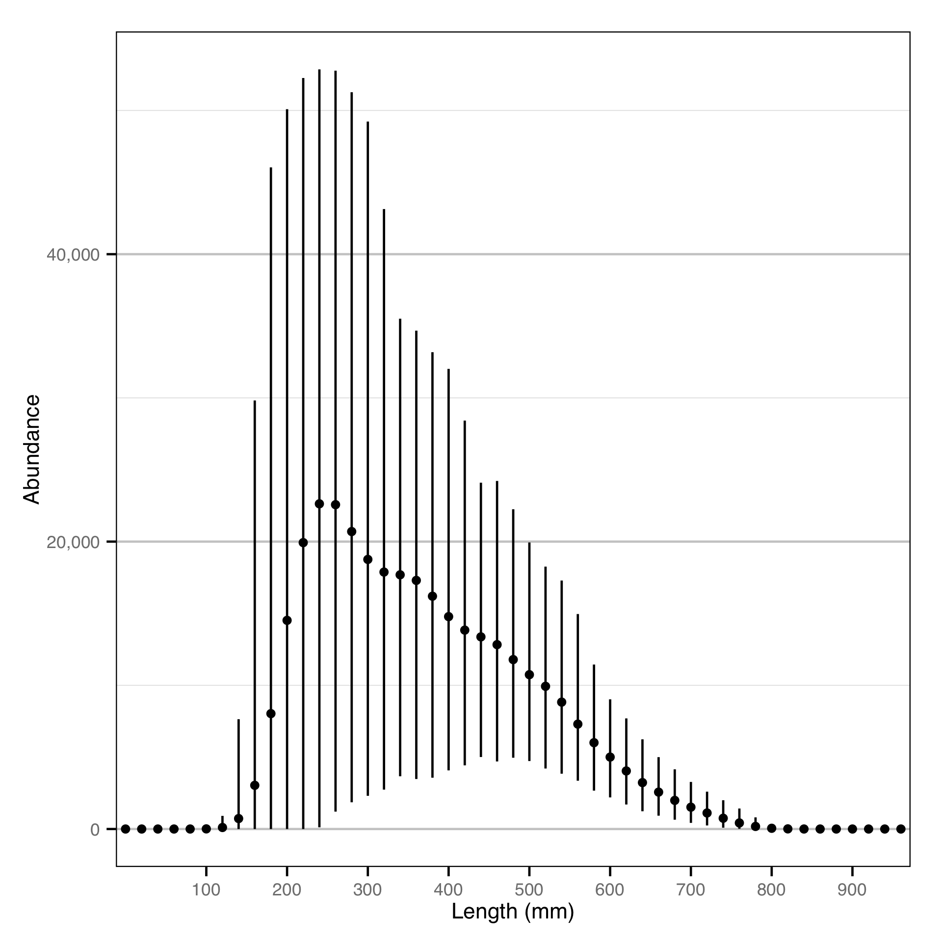
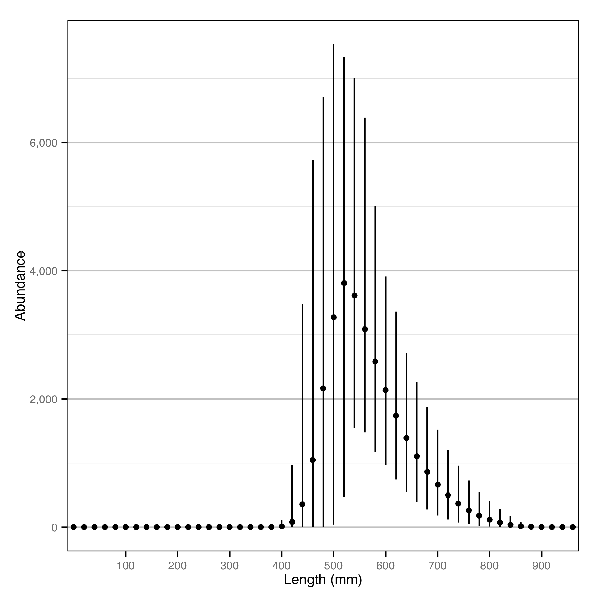
Finally, the abundance by age-class estimates are converted into abundance by length-class estimates assuming a von Bertalanffy growth curve. The growth parameters for Gerrard Rainbow Trout will be taken from Thorley (Thorley 2015); the growth parameters for Bull Trout will be assumed to be the same.
Data Preparation
The parameters used for the analysis must be provided as two files located in the folder .\input\. The abdunace parameters used in this analysis, which must be in the file .\input\parameters.csv, are:
| species | parameter | estimate | lower | upper | sd |
|---|---|---|---|---|---|
| RB | N_S | NA | NA | NA | NA |
| RB | sigma | NA | NA | NA | NA |
| RB | N_C | 8637.00 | 7.0e+03 | 1.00e+04 | 1000.00 |
| RB | gamma | 0.13 | 8.0e-02 | 1.90e-01 | 0.03 |
| RB | omega_A | 0.48 | 3.6e-01 | 6.30e-01 | 0.06 |
| RB | N_1 | 126000.00 | 9.7e+04 | 1.63e+05 | 16900.00 |
| RB | lambda | 9.00 | NA | NA | NA |
| BT | N_S | NA | NA | NA | NA |
| BT | sigma | NA | NA | NA | NA |
| BT | N_C | 4845.00 | 4.0e+03 | 6.00e+03 | 500.00 |
| BT | gamma | 0.17 | 1.1e-01 | 2.40e-01 | 0.03 |
| BT | omega_A | 0.48 | 3.5e-01 | 6.30e-01 | 0.07 |
| BT | N_1 | NA | NA | NA | NA |
| BT | lambda | 14.00 | NA | NA | NA |
The von Bertalanffy growth parameters used in this analysis, which must be in the file .\input\vB.csv, are:
| species | parameter | estimate | lower | upper | sd |
|---|---|---|---|---|---|
| RB | bK | 0.17204 | 0.15224 | 0.19128 | 0.01034 |
| RB | bLInf | 924.18000 | 904.69000 | 951.64000 | 11.83000 |
| RB | sLength | 20.59600 | 17.63400 | 23.95700 | 1.54000 |
| RB | t0 | -0.85200 | -1.64400 | -0.28300 | 0.34900 |
| BT | bK | 0.17204 | 0.15224 | 0.19128 | 0.01034 |
| BT | bLInf | 924.18000 | 904.69000 | 951.64000 | 11.83000 |
| BT | sLength | 20.59600 | 17.63400 | 23.95700 | 1.54000 |
| BT | t0 | -0.85200 | -1.64400 | -0.28300 | 0.34900 |
These files may be modified at will, with parameters added or removed as appropriate; the code will check that the structure is correct for each species and for both sets of spawner and catch parameters, and will run the analysis and produce plots for each valid combination. Additional fish species may also be added to the end of the input files, provided the structure is identical to the above.
Statistical Analysis
Bayesian models were fitted to the data using R version 3.2.1 (Team 2013) and JAGS 3.4.0 (Plummer 2012) which interfaced with each other via jaggernaut 2.3.0 (Thorley 2013). For additional information on Bayesian modelling in the BUGS language, of which JAGS uses a dialect, the reader is referred to Kery and Schaub (2011, 41–44).
Unless indicated otherwise, the models use prior distributions in the form of a normal distribution defined by the parameters provided for the analysis, truncated by the lower and upper credible limits. The posterior distributions were estimated from a minimum of 1,000 Markov Chain Monte Carlo (MCMC) samples thinned from the second halves of three chains (Kery and Schaub 2011, 38–40). Model convergence was confirmed by ensuring that Rhat (Kery and Schaub 2011, 40) was less than 1.1 for each of the parameters in the model (Kery and Schaub 2011, 61).
The posterior distributions of the parameters are summarised in terms of a point estimate (mean), lower and upper 95% credible limits (2.5th and 97.5th percentiles), the standard deviation (SD), percent relative error (half the 95% credible interval as a percent of the point estimate) and significance (Kery and Schaub 2011, 37, 42).
The results are displayed graphically by plotting the modeled relationships between particular variables and the response with 95% credible intervals (CRIs) with the remaining variables held constant.
Model Code
The JAGS model code, which uses a series of naming conventions, is presented below.
Abundance
Abundance - Model1
model{

    bN ~ dnorm(N.mean, N.sd^-2) T(N.lower, N.upper)
    bP ~ dnorm(p.mean, p.sd^-2) T(p.lower, p.upper)

    N_A <- bN/bP

    bOmega_A ~ dnorm(omega_A.mean, omega_A.sd^-2) T(omega_A.lower, omega_A.upper)

    N_4 <- N_A * ((bOmega_A - 1) * bOmega_A^3)/(bOmega_A^iLambda - bOmega_A^3)

    for(i in 4:iLambda){
      N[i] <- N_4 * bOmega_A^(i-4)
    }

    N_1 ~ dnorm(N_1.mean, N_1.sd^-2) T(N_1.lower, N_1.upper)

    bOmega_J <- ifelse(N_1 == 1, 0, (N_4/N_1)^(1/3))

    for(i in 1:3){
      N[i] <- ifelse(N_1 == 1, 0, N_1 * bOmega_J^(i-1))
    }
}
Results
Model Parameters
The posterior distributions for the fixed (Kery and Schaub 2011 p. 75) parameters in each model are summarised below.
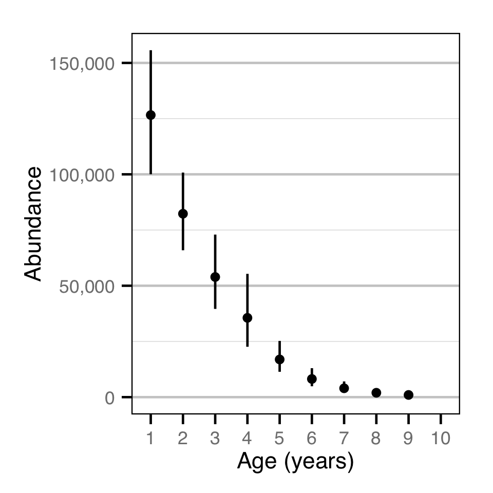
Abundance - Rainbow Trout - Catch
| Parameter | Estimate | Lower | Upper | SD | Error | Significance |
|---|---|---|---|---|---|---|
| N_A | 67590 | 45590 | 101190 | 14610 | 41 | 7e-04 |
| N[1] | 126600 | 100040 | 155700 | 14650 | 22 | 7e-04 |
| N[2] | 82310 | 65920 | 100790 | 8980 | 21 | 7e-04 |
| N[3] | 53920 | 39600 | 72960 | 8680 | 31 | 7e-04 |
| N[4] | 35590 | 22610 | 55340 | 8440 | 46 | 7e-04 |
| N[5] | 16920 | 11380 | 25230 | 3670 | 41 | 7e-04 |
| N[6] | 8151 | 4888 | 13002 | 2094 | 50 | 7e-04 |
| N[7] | 3979 | 1953 | 7055 | 1329 | 64 | 7e-04 |
| N[8] | 1968 | 753 | 4000 | 843 | 83 | 7e-04 |
| N[9] | 985 | 292 | 2278 | 523 | 100 | 7e-04 |
| Convergence | Iterations |
|---|---|
| 1 | 1000 |
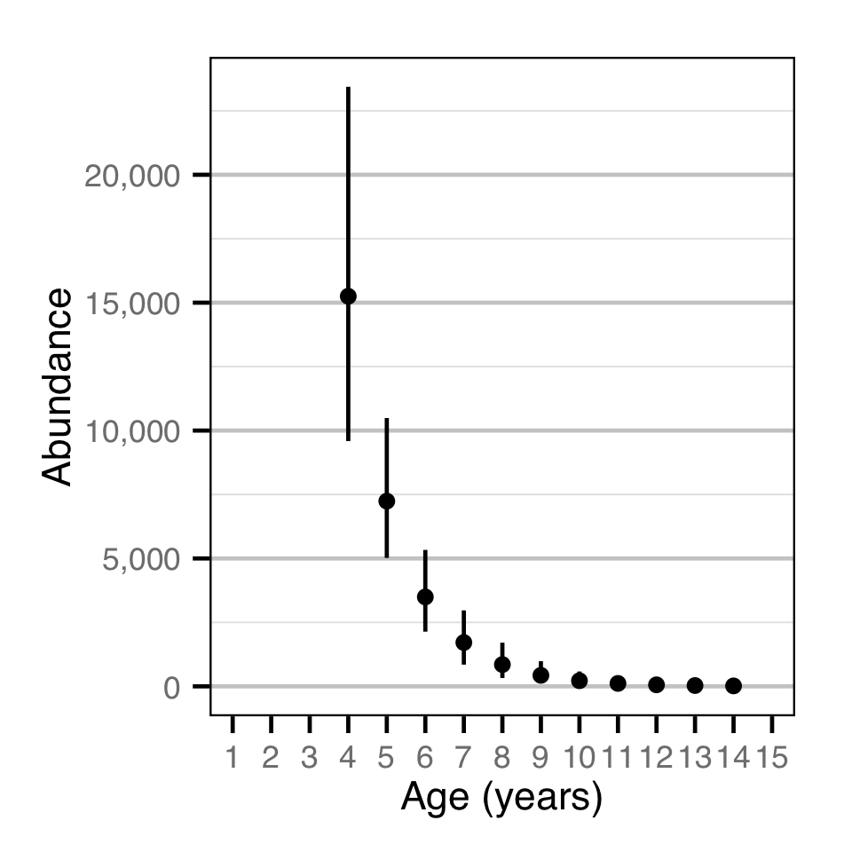
Abundance - Bull Trout - Catch
| Parameter | Estimate | Lower | Upper | SD | Error | Significance |
|---|---|---|---|---|---|---|
| N_A | 29420.00 | 20460.00 | 42620.00 | 5740.00 | 38 | 7e-04 |
| N[10] | 219.80 | 45.20 | 580.50 | 144.10 | 120 | 7e-04 |
| N[11] | 113.90 | 16.50 | 349.10 | 88.40 | 150 | 7e-04 |
| N[12] | 59.70 | 6.10 | 207.00 | 53.80 | 170 | 7e-04 |
| N[13] | 31.60 | 2.20 | 126.70 | 32.50 | 200 | 7e-04 |
| N[14] | 16.96 | 0.82 | 75.23 | 19.63 | 220 | 7e-04 |
| N[4] | 15250.00 | 9590.00 | 23440.00 | 3520.00 | 45 | 7e-04 |
| N[5] | 7241.00 | 5021.00 | 10490.00 | 1412.00 | 38 | 7e-04 |
| N[6] | 3495.00 | 2138.00 | 5334.00 | 820.00 | 46 | 7e-04 |
| N[7] | 1713.00 | 849.00 | 2969.00 | 549.00 | 62 | 7e-04 |
| N[8] | 852.00 | 326.00 | 1706.00 | 362.00 | 81 | 7e-04 |
| N[9] | 429.80 | 121.90 | 982.40 | 231.20 | 100 | 7e-04 |
| Convergence | Iterations |
|---|---|
| 1.01 | 1000 |
Figures
Abundance - Rainbow Trout - Catch


Abundance - Bull Trout - Catch


Length - Rainbow Trout - Catch

Length - Bull Trout - Catch

Acknowledgements
The organisations and individuals whose contributions have made this analysis report possible include:
- Redfish Consulting
- Greg Andrusak
References
Kery, Marc, and Michael Schaub. 2011. Bayesian Population Analysis Using WinBUGS : A Hierarchical Perspective. Boston: Academic Press. http://www.vogelwarte.ch/bpa.html.
Plummer, Martyn. 2012. “JAGS Version 3.3.0 User Manual.” http://sourceforge.net/projects/mcmc-jags/files/Manuals/3.x/.
Team, R Core. 2013. “R: A Language and Environment for Statistical Computing.” Vienna, Austria: R Foundation for Statistical Computing. http://www.R-project.org.
Thorley, J. L. 2013. “Jaggernaut: An R Package to Facilitate Bayesian Analyses Using JAGS (Just Another Gibbs Sampler).” Nelson, B.C.: Poisson Consulting Ltd. https://github.com/poissonconsulting/jaggernaut.
———. 2014. “Kootenay Lake Exploitation Study 2013.” Poisson Consulting Analysis Report. https://www.poissonconsulting.ca/f/1088509848.
———. 2015. “Kootenay Lake Gerrard Rainbow Trout Condition and Growth Analysis 2014.” Poisson Consulting Analysis Report. https://www.poissonconsulting.ca/f/723490014.