Lower Columbia River Rainbow Trout Spawning Analysis 2014
The suggested citation for this analytic report is:
Thorley, J.L. (2015) Lower Columbia River Rainbow Trout Spawning Analysis 2014. A Poisson Consulting Analysis Report. URL: https://www.poissonconsulting.ca/f/1157179155.
Background
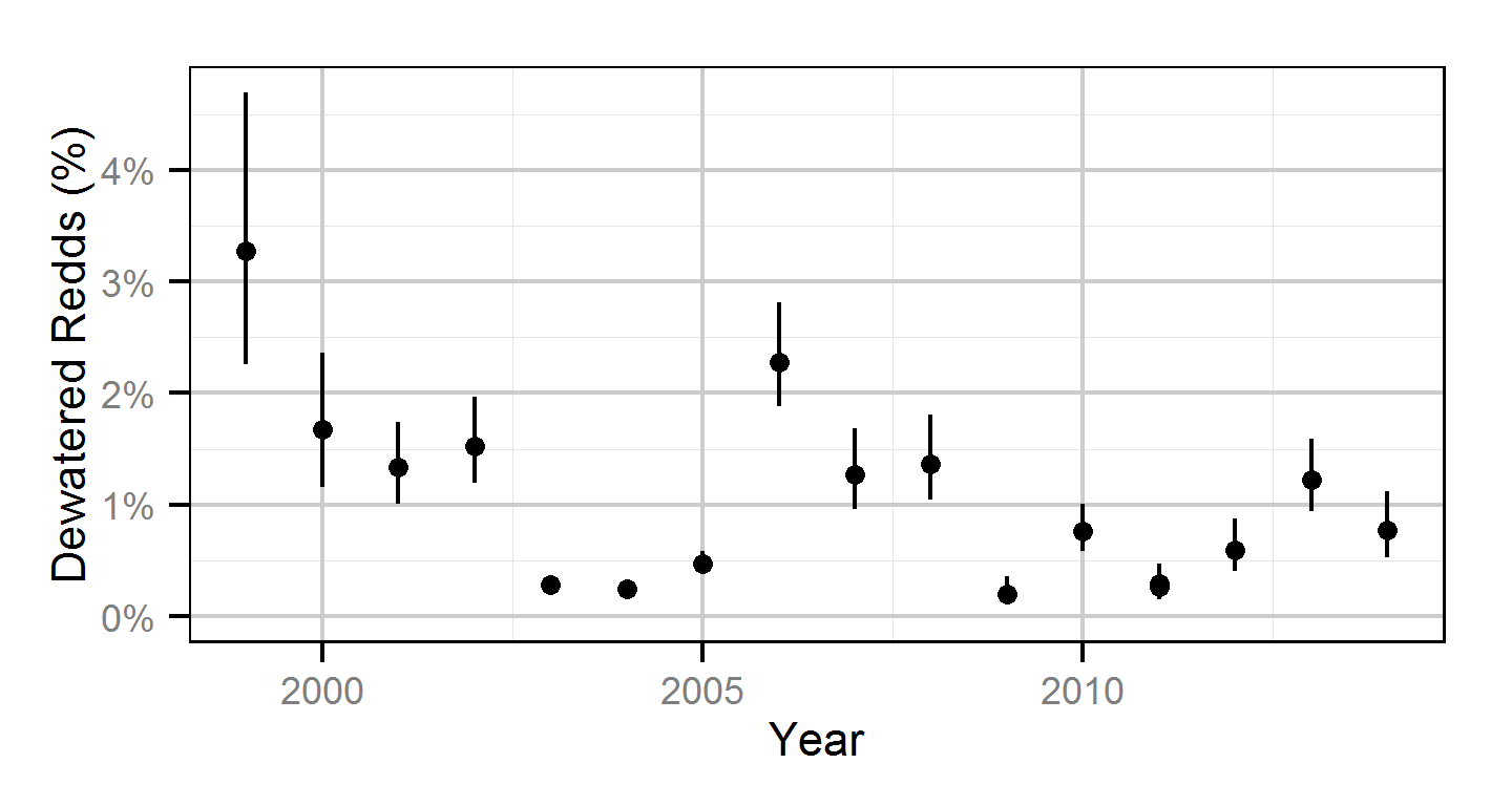
Each spring in the Lower Columbia River (LCR) below Hugh L. Keenleyside Dam (HLK) and in the Lower Kootenay River (LKR) below Brilliant Dam, thousands of Rainbow Trout spawn. Since 1992, BC Hydro has stabilized the spring discharge releases from HLK to protect Rainbow Trout redds from dewatering.
The primary goal of the current analysis to answer the following management question:
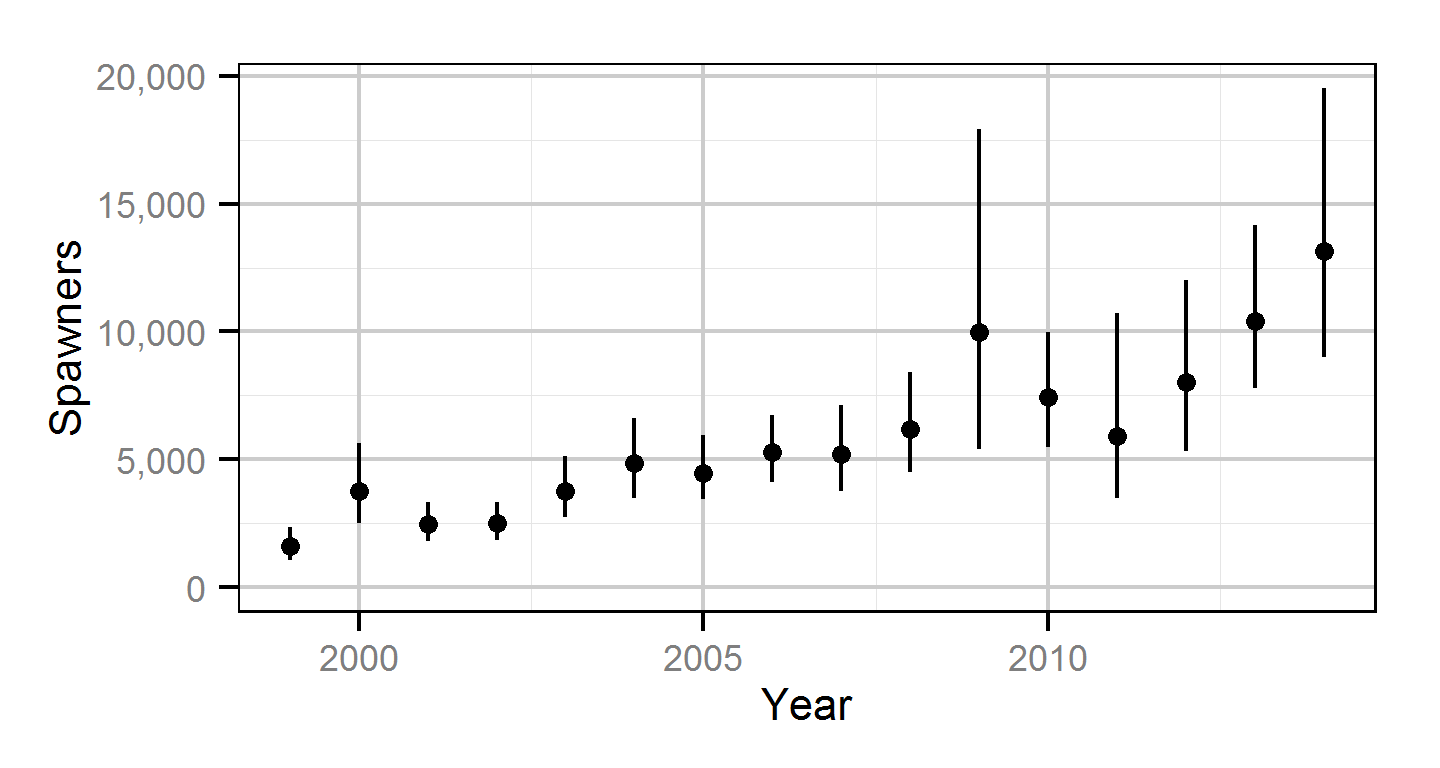
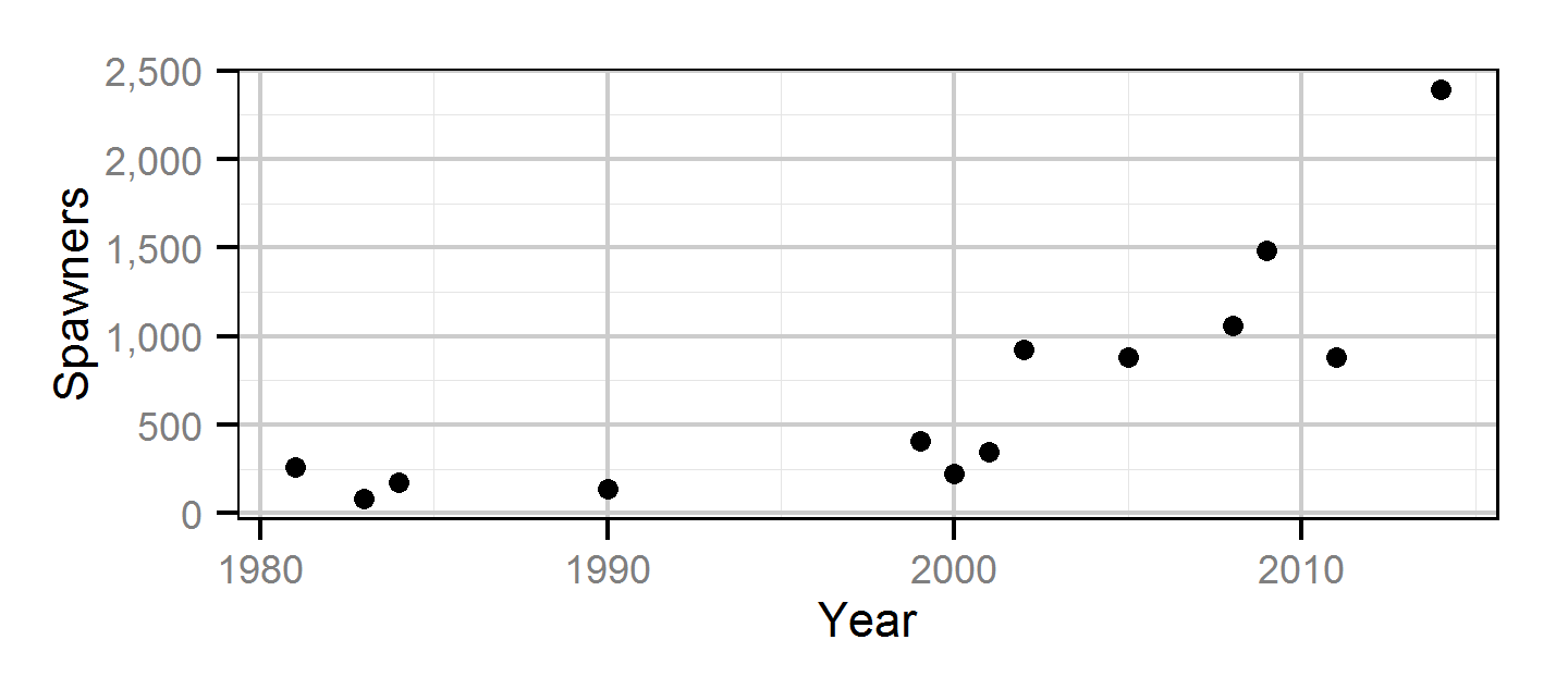
Does the implementation of Rainbow Trout Spawning Protection Flows over the course of the monitoring period lead to an increase in the relative abundance of Rainbow Trout spawning in the LCR downstream of HLK dam?
Methods
Data Preparation
The Rainbow Trout fish and redd aerial count data for the LCR and LKR were collected by Mountain Water Research and databased by Gary Pavan. The age-1 Rainbow Trout abundance data were provided by the Fish Population Indexing Program which is led by Golder Associates.
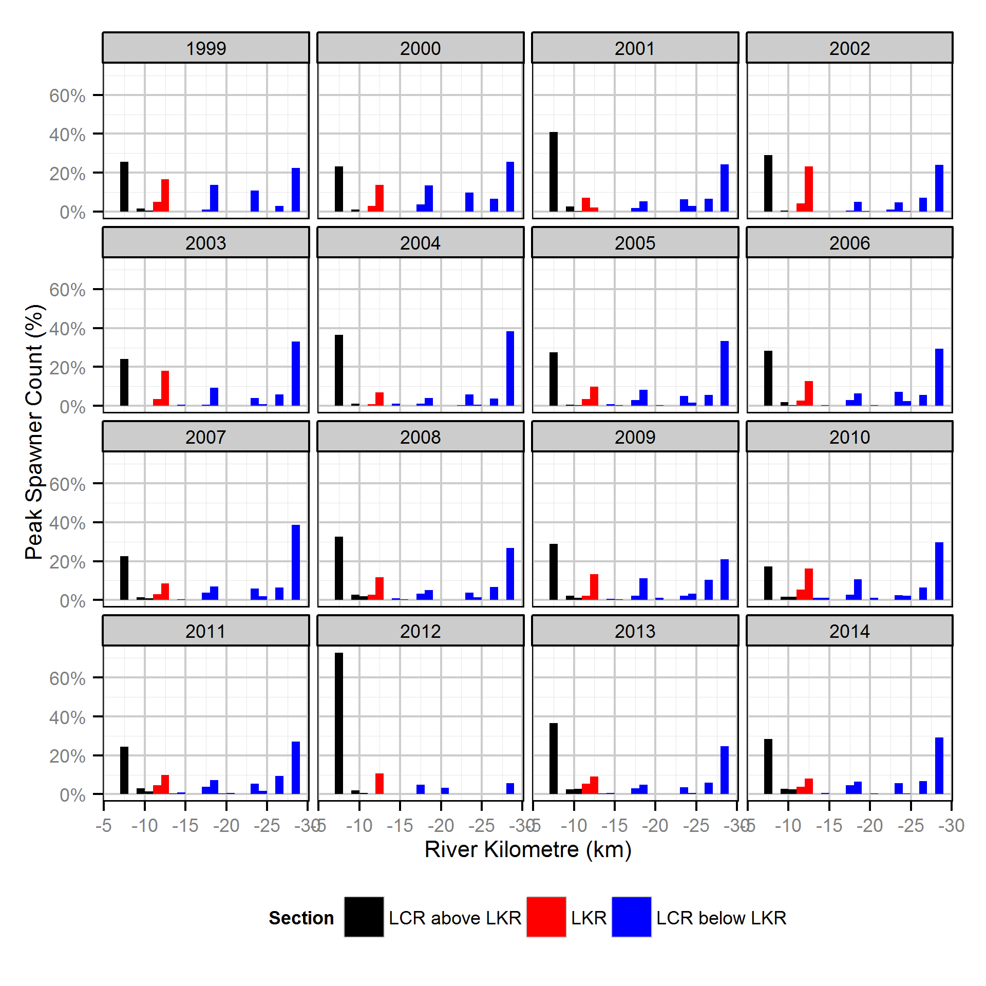
The study area was divided into three sections: the LCR above the LKR, the LKR and the LCR below the LKR. Redd and spawner counts upstream of Norns Creek Fan and downstream of Genelle were excluded from the section totals because they constitute less than 0.1% of the total count and were not surveyed in all years. The redd and spawner counts for the Right Upstream Bank above Robson Bridge were also excluded as they appear to be primarily driven by viewing conditions (and consitute less than 2.5% of the total). Simultaneous declines in both spawners and redds for a particular section were inferred to be caused by poor viewing conditions (turbidity) and the affected spawner and redd section counts were excluded from any subsequent analyses.
Statistical Analysis
Hierarchical Bayesian models were fitted to the count data using R version 3.1.1 (Team, 2013) and JAGS 3.4.0 (Plummer, 2012) which interfaced with each other via jaggernaut 1.8.2 . For additional information on hierarchical Bayesian modelling in the BUGS language, of which JAGS uses a dialect, the reader is referred to Kery and Schaub (2011) pages 41-44.
Unless specified, the models assumed vague (low information) prior distributions . The posterior distributions were estimated from a minimum of 1,000 Markov Chain Monte Carlo (MCMC) samples thinned from the second halves of three chains . Model convergence was confirmed by ensuring that Rhat was less than 1.1 for each of the parameters in the model . Model adequacy was confirmed by examination of residual plots.
The posterior distributions of the fixed parameters are summarised in terms of a point estimate (mean), lower and upper 95% credible limits (2.5th and 97.5th percentiles), the standard deviation (SD), percent relative error (half the 95% credible interval as a percent of the point estimate) and significance .
Model selection was achieved by dropping insignificant explanatory parameters and uninformative hyperparameters. For the purposes of the current analysis an explanatory parameter was considered to be insignificant if its significance was \(\geq\) 0.05 and a hyperparameter was considered to be uninformative if its percent relative error was \(\geq\) 80%.
The results are displayed graphically by plotting the modeled relationships between particular variables and the response with 95% credible intervals (CRIs) with the remaining variables held constant. In general, continuous and discrete fixed variables are held constant at their mean and first level values respectively while random variables are held constant at their typical values (expected values of the underlying hyperdistributions) . Where informative the influence of particular variables is expressed in terms of the effect size (i.e., percent change in the response variable) with 95% CRIs (Bradford, Korman, and Higgins, 2005). Plots were produced using the ggplot2 R package .
Area-Under-the-Curve
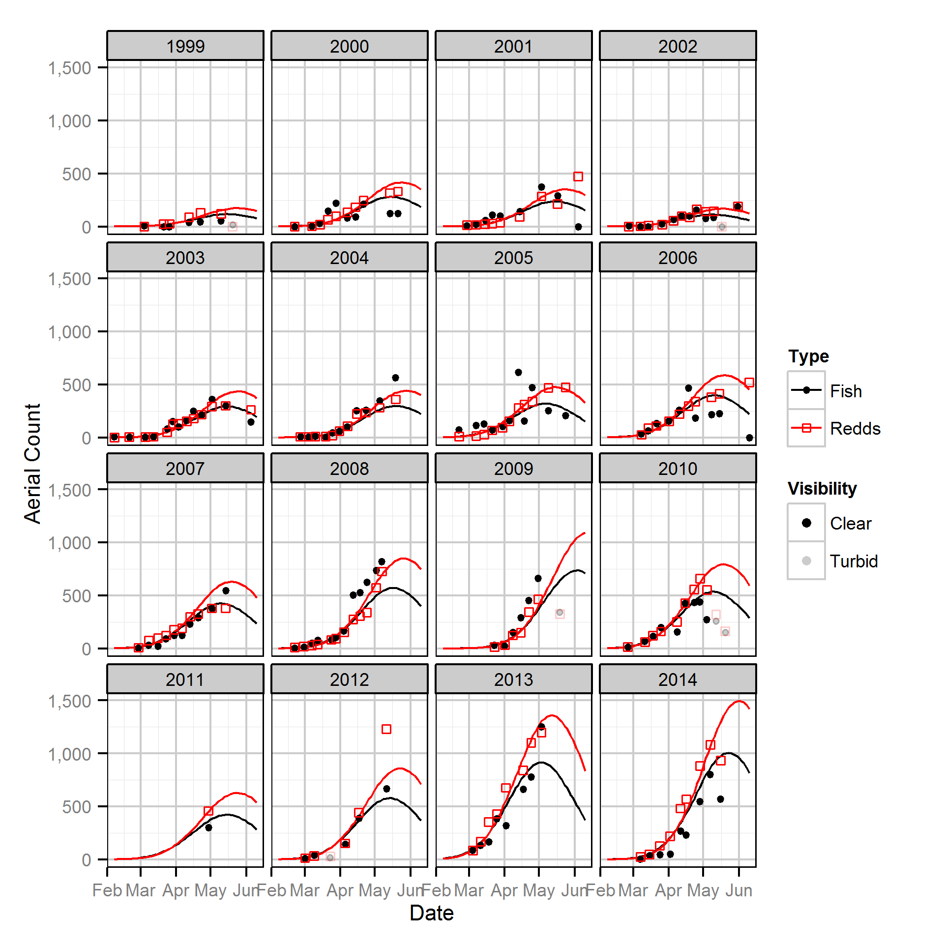
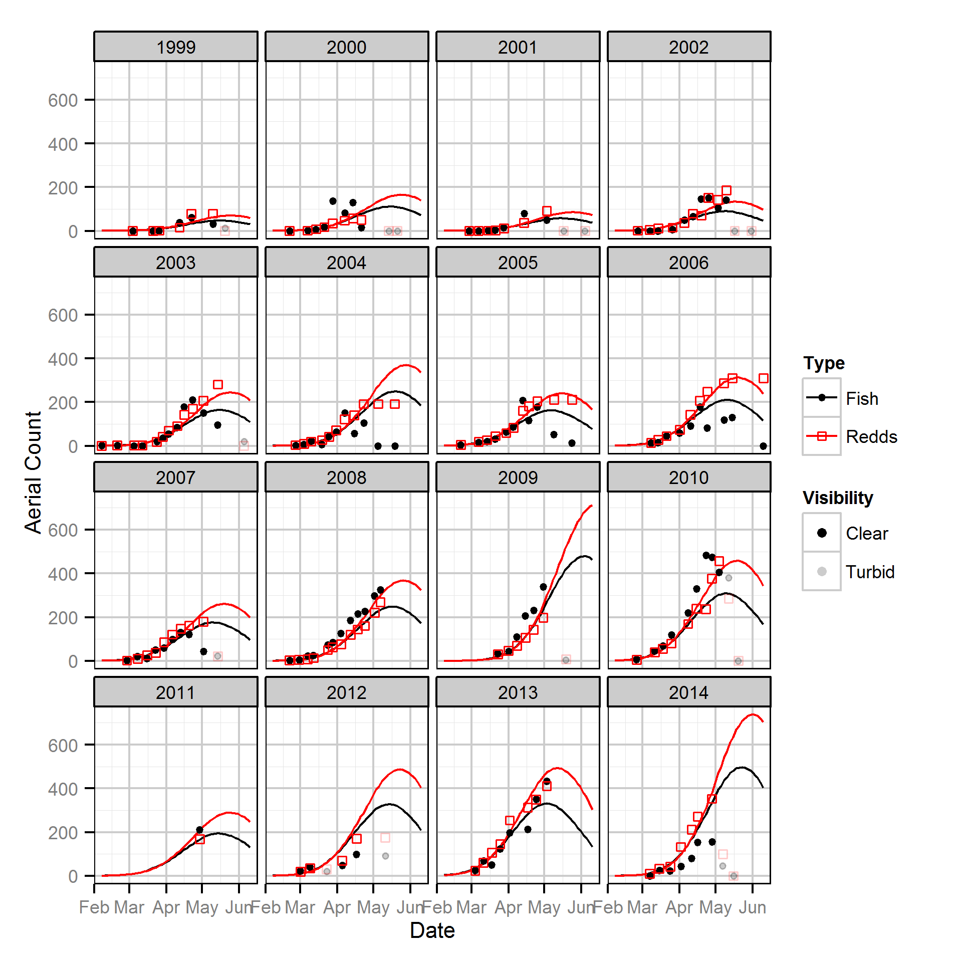
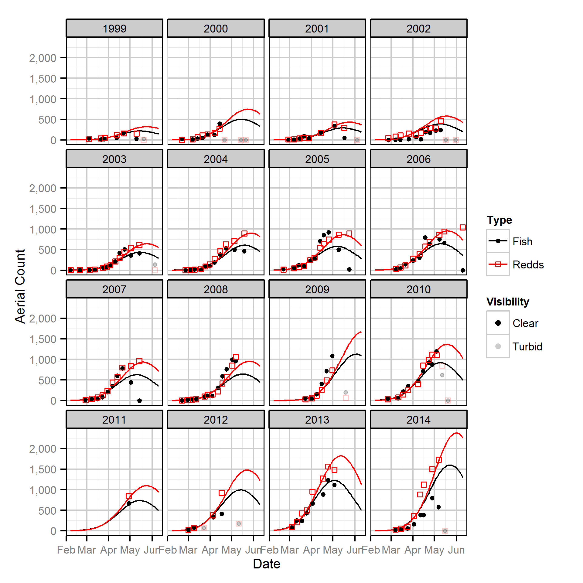
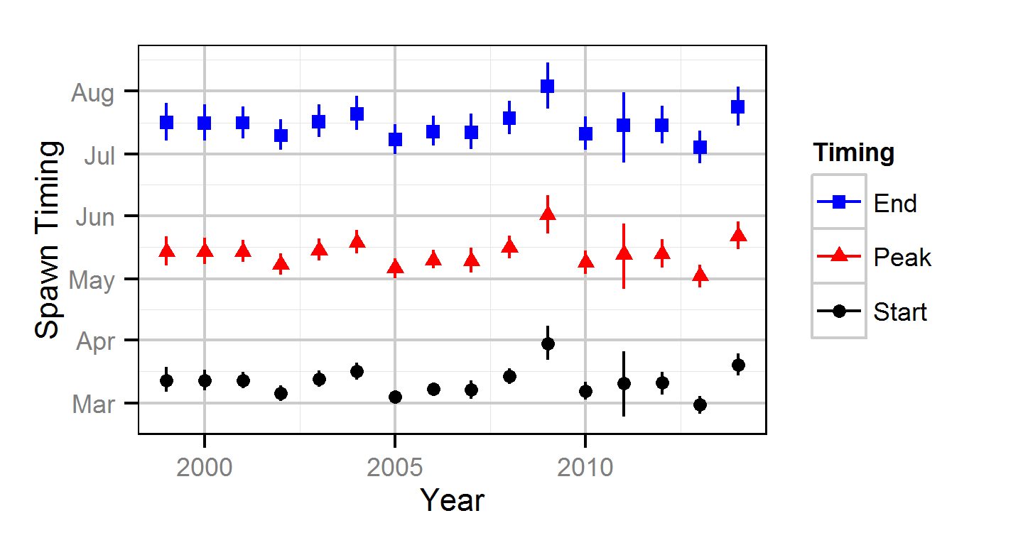
The spawner abundance and spawn timing was estimated from the aerial fish and redd counts for the three sections using an Area-Under-the-Curve (AUC) model.
Key assumptions of the AUC model include:
- Abundance varies by section.
- Abundance varies randomly by year and section within year.
- Spawner observer efficiency is between 0.9 and 1.1.
- Redd observer efficiency is 1.0.
- Mean spawner residence time is between 14 and 21 days.
- Redd residence time is 35 days.
- The number of redds per spawer is a fixed constant.
- Spawner and redd arrival and departure are normally distributed.
- The duration of spawning is constant across years.
- Peak spawn timing varies randomly by year.
- The residual variation in the spawner and redd counts is described by overdispersed Poisson distributions (Poisson-gamma distributions).
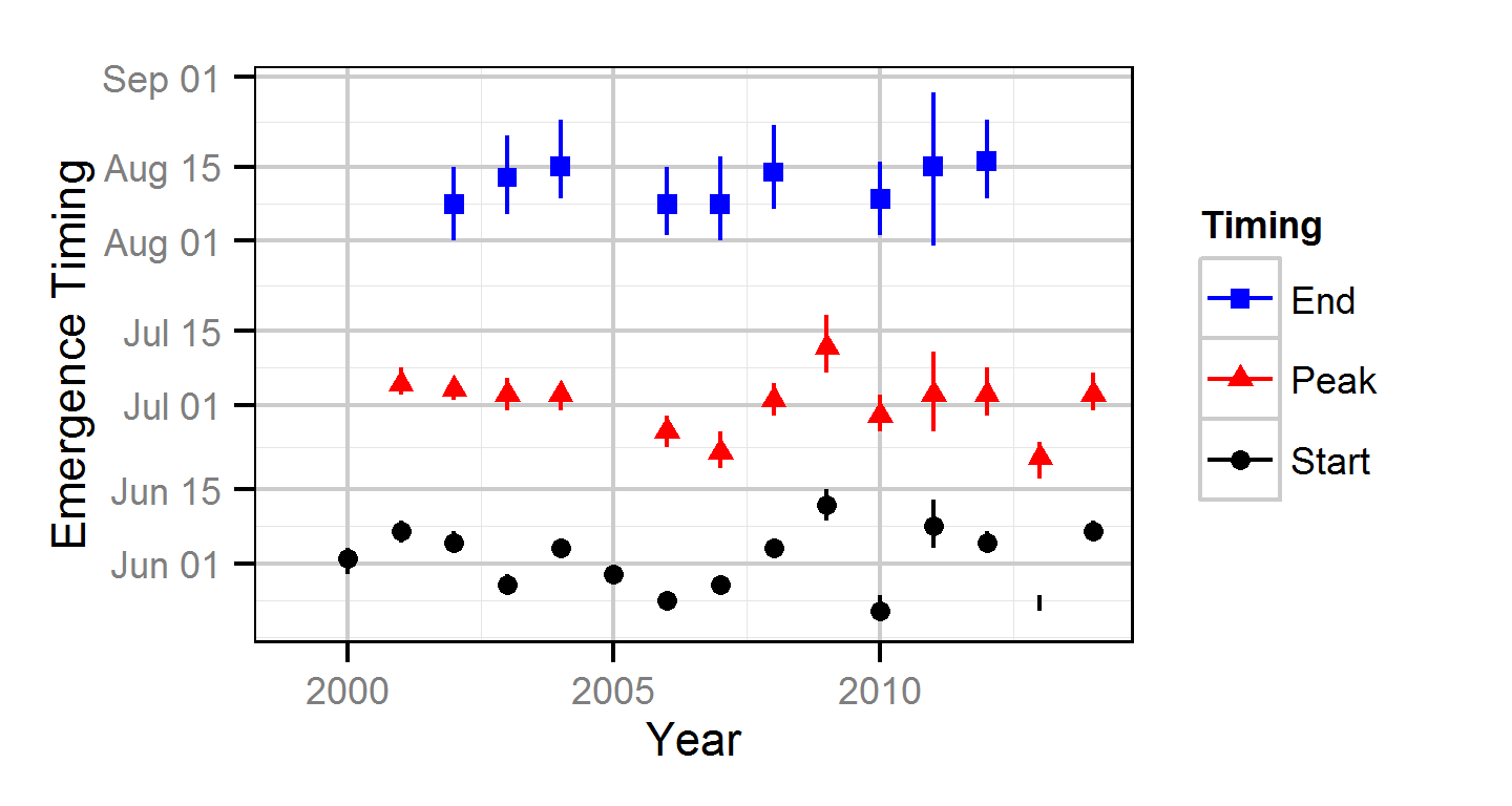
The expected emergence timing was calculated from the estimated spawn timing and the surface water temperature under the assumption that Rainbow Trout embryos emerge after 480 accumulated thermal units (ATUs).
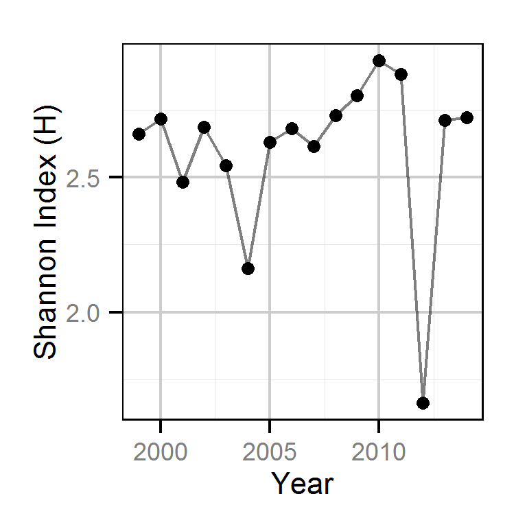
The proportions of spawners at each site were used to calculate the Shannon Index, an information-theoretic measure of the diversity in the abundance distribution of a resource (Krebs, 1999). In the current context, the Shannon Index takes into account both the number of spawning sites and how the spawning activity is distributed among these, with a higher index indicating a greater spatial distribution of spawning.
The Shannon Index (\(H\)) is given by \[ H = - \sum{p_i log(p_i)}\] where \(p_i\) is the proportion of the spawning activity at the ith location.
Stock-Recruitment
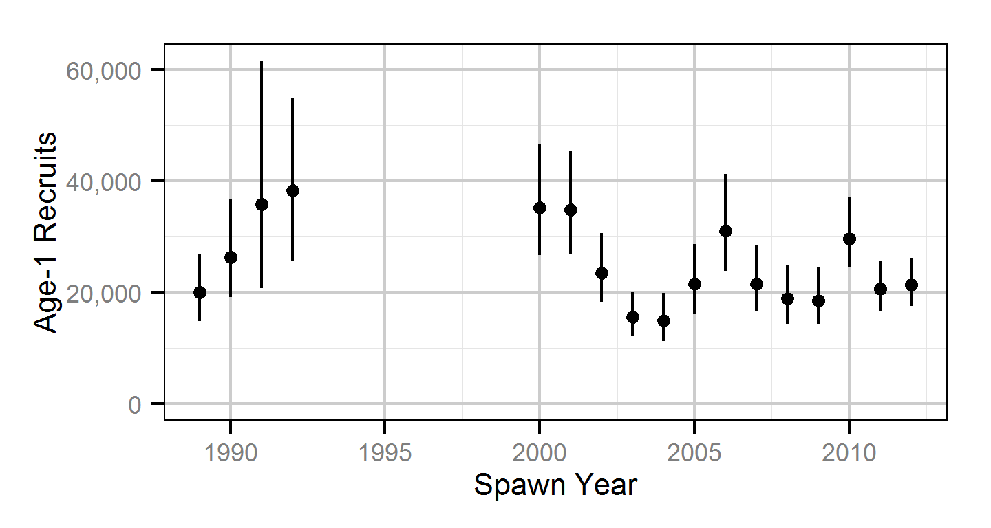
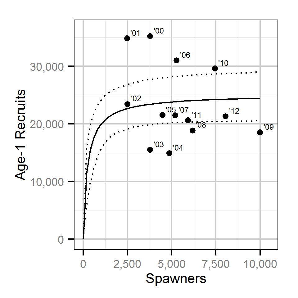
The relationship between the number of spawners and the number of age-1 recruits in the fall of the following year was estimated using a Beverton-Holt stock-recruitment model.
Key assumptions of the stock-recruitment model include:
- The prior probability distribution for the maximum number of recruits per spawner (
R0) is normally distributed with a mean of 90 and a SD of 50. - The residual variation in the number of age-1 recruits is log-normally distributed.
The prior probability distribution mean of 90 for R0 was based on an average of 2,900 eggs per female spawner, a 50:50 sex ratio, 50% egg survival, 50% post-emergence fall survival, 50% overwintering survival and 50% summer survival.
Model Code
The JAGS model code, which uses a series of naming conventions, is presented below.
Area-Under-The-Curve
| Variable/Parameter | Description |
|---|---|
bPeakSpawnerArrivalTiming |
Timing of peak of spawner arrival |
bReddObserverEfficiency |
Redd observer efficiency |
bReddPerSpawner |
Number of redds per spawner |
bReddResidenceTime |
Redd residence time |
bSpawnerAbundanceSite[i] |
Intercept for spawner abundance at ith site |
bSpawnerObserverEfficiency |
Spawner observer efficiency |
bSpawnerResidenceTime |
Spawner residence time |
Dayte[i] |
Day of the year of the ith count |
Fish[i] |
Number of fish observed on ith count |
Redds[i] |
Number of redds observed on ith count |
sFishDispersion |
SD of overdispersion for Fish |
Site[i] |
Site of the ith count |
sPeakSpawnerArrivalTimingYear |
SD of effect of Year on bPeakSpawnerArrivalTiming |
sReddsDispersion |
SD of overdispersion for Redds |
sSpawnDuration |
SD of the duration of spawning |
sSpawnerAbundanceSiteYear |
SD of effect of Site within Year on bSpawnerAbundanceSite |
sSpawnerAbundanceYear |
SD of effect of Year on bSpawnerAbundanceSite |
Year[i] |
Year of the ith count |
Area-Under-The-Curve - Model1
model {

  sSpawnDuration ~ dunif(14, 42)

  bPeakSpawnerArrivalTiming ~ dnorm(130, 14^-2)

  bSpawnerResidenceTime ~ dunif(14, 21)
  bSpawnerObserverEfficiency ~ dunif(0.9, 1.1)

  bReddObserverEfficiency ~ dunif(0.9, 1.1)
  bReddResidenceTime <- 35

  bReddPerSpawner ~ dunif(0, 4)

  sPeakSpawnerArrivalTimingYear ~ dunif(0, 28)
  sSpawnerAbundanceYear ~ dunif(0, 2)
  for (i in 1:nYear) {
    bPeakSpawnerArrivalTimingYear[i] ~ dnorm (0, sPeakSpawnerArrivalTimingYear^-2)
    bSpawnerAbundanceYear[i] ~ dnorm (0, sSpawnerAbundanceYear^-2)
  }

  sSpawnerAbundanceSiteYear ~ dunif (0, 2)
  for (i in 1:nSite) {
    bSpawnerAbundanceSite[i] ~ dnorm (5, 5^-2)
    for (j in 1:nYear) {
      bSpawnerAbundanceSiteYear[i, j] ~ dnorm (0, sSpawnerAbundanceSiteYear^-2)
    }
  }

  sFishDispersion ~ dunif(0, 2)
  sReddDispersion ~ dunif(0, 2)
  for (i in 1:length(Fish)) {
    ePeakSpawnerArrivalTiming[i] <- bPeakSpawnerArrivalTiming + bPeakSpawnerArrivalTimingYear[Year[i]]

    log(eSpawnerAbundance[i]) <- bSpawnerAbundanceSite[Site[i]] + bSpawnerAbundanceYear[Year[i]] + bSpawnerAbundanceSiteYear[Site[i], Year[i]]

    eFish[i] <- (pnorm(Dayte[i], ePeakSpawnerArrivalTiming[i], sSpawnDuration^-2) - pnorm(Dayte[i], ePeakSpawnerArrivalTiming[i] + bSpawnerResidenceTime, sSpawnDuration^-2)) * eSpawnerAbundance[i] * bSpawnerObserverEfficiency

    eRedds[i] <- (pnorm(Dayte[i], ePeakSpawnerArrivalTiming[i], sSpawnDuration^-2) - pnorm(Dayte[i], ePeakSpawnerArrivalTiming[i] + bReddResidenceTime, sSpawnDuration^-2)) * eSpawnerAbundance[i] * bReddPerSpawner * bReddObserverEfficiency

    eFishDispersion[i] ~ dgamma(1 / sFishDispersion^2, 1 / sFishDispersion^2)
    eReddDispersion[i] ~ dgamma(1 / sReddDispersion^2, 1 / sReddDispersion^2)

    Fish[i] ~ dpois(eFish[i] *  eFishDispersion[i])
    Redds[i] ~ dpois(eRedds[i] *  eReddDispersion[i])
  }
}
Stock-Recruitment
| Variable/Parameter | Description |
|---|---|
eRecruits |
Expected number of Recruits |
k |
Maximum Recruits |
R0 |
Maximum Recruits per Stock |
Recruits |
Number of age-1 individuals the following year |
sRecruits |
SD of log-normally distributed residual variation in Recruits |
Stock |
Number of spawners |
Stock-Recruitment - Model1
model {

  R0 ~ dnorm(2900 * 0.5^5, 50^-2) T(0, )

  k ~ dlnorm(10, 5^-2)

  sRecruits ~ dunif(0, 5)
  for (i in 1:length(Stock)) {
    eRecruits[i] <- R0 * Stock[i] / (1 + Stock[i] * (R0 - 1) / k)
    Recruits[i] ~ dlnorm(log(eRecruits[i]), sRecruits^-2)
  }
}
Results
Model Parameters
The posterior distributions for the fixed (Kery and Schaub 2011 p. 75) parameters in each model are summarised below.
Area-Under-The-Curve
| Parameter | Estimate | Lower | Upper | SD | Error | Significance |
|---|---|---|---|---|---|---|
| bPeakSpawnerArrivalTiming | 126.1914 | 120.9502 | 131.8695 | 2.7488 | 4 | 0 |
| bReddObserverEfficiency | 0.9955 | 0.9046 | 1.0934 | 0.0561 | 9 | 0 |
| bReddPerSpawner | 0.7661 | 0.6157 | 0.9294 | 0.0851 | 20 | 0 |
| bReddResidenceTime | 35.0000 | 35.0000 | 35.0000 | 0.0000 | 0 | 0 |
| bSpawnerAbundanceSite[1] | 7.3473 | 6.9451 | 7.7525 | 0.2086 | 5 | 0 |
| bSpawnerAbundanceSite[2] | 6.6450 | 6.2269 | 7.0652 | 0.2122 | 6 | 0 |
| bSpawnerAbundanceSite[3] | 7.8584 | 7.4406 | 8.2831 | 0.2117 | 5 | 0 |
| bSpawnerObserverEfficiency | 1.0061 | 0.9060 | 1.0948 | 0.0564 | 9 | 0 |
| bSpawnerResidenceTime | 17.0225 | 14.1652 | 20.5962 | 1.8557 | 19 | 0 |
| sFishDispersion | 0.7832 | 0.7241 | 0.8411 | 0.0303 | 7 | 0 |
| sPeakSpawnerArrivalTimingYear | 8.2512 | 5.3229 | 13.1978 | 2.0025 | 48 | 0 |
| sReddDispersion | 0.2851 | 0.2589 | 0.3135 | 0.0144 | 10 | 0 |
| sSpawnDuration | 27.8910 | 26.6355 | 29.2164 | 0.6708 | 5 | 0 |
| sSpawnerAbundanceSiteYear | 0.2206 | 0.1575 | 0.3013 | 0.0373 | 33 | 0 |
| sSpawnerAbundanceYear | 0.6642 | 0.4296 | 1.0110 | 0.1593 | 44 | 0 |
| Rhat | Iterations |
|---|---|
| 1.02 | 8e+05 |
Stock-Recruitment
| Parameter | Estimate | Lower | Upper | SD | Error | Significance |
|---|---|---|---|---|---|---|
| k | 2.350e+04 | 1.971e+04 | 2.750e+04 | 2009.0000 | 17 | 0 |
| R0 | 1.084e+02 | 3.689e+01 | 2.012e+02 | 43.1080 | 76 | 0 |
| sRecruits | 3.208e-01 | 2.157e-01 | 4.815e-01 | 0.0706 | 41 | 0 |
| Rhat | Iterations |
|---|---|
| 1.09 | 10000 |
Figures
Discharge
Temperature
Acoustic Detections

Area-Under-The-Curve
Stock-Recruitment
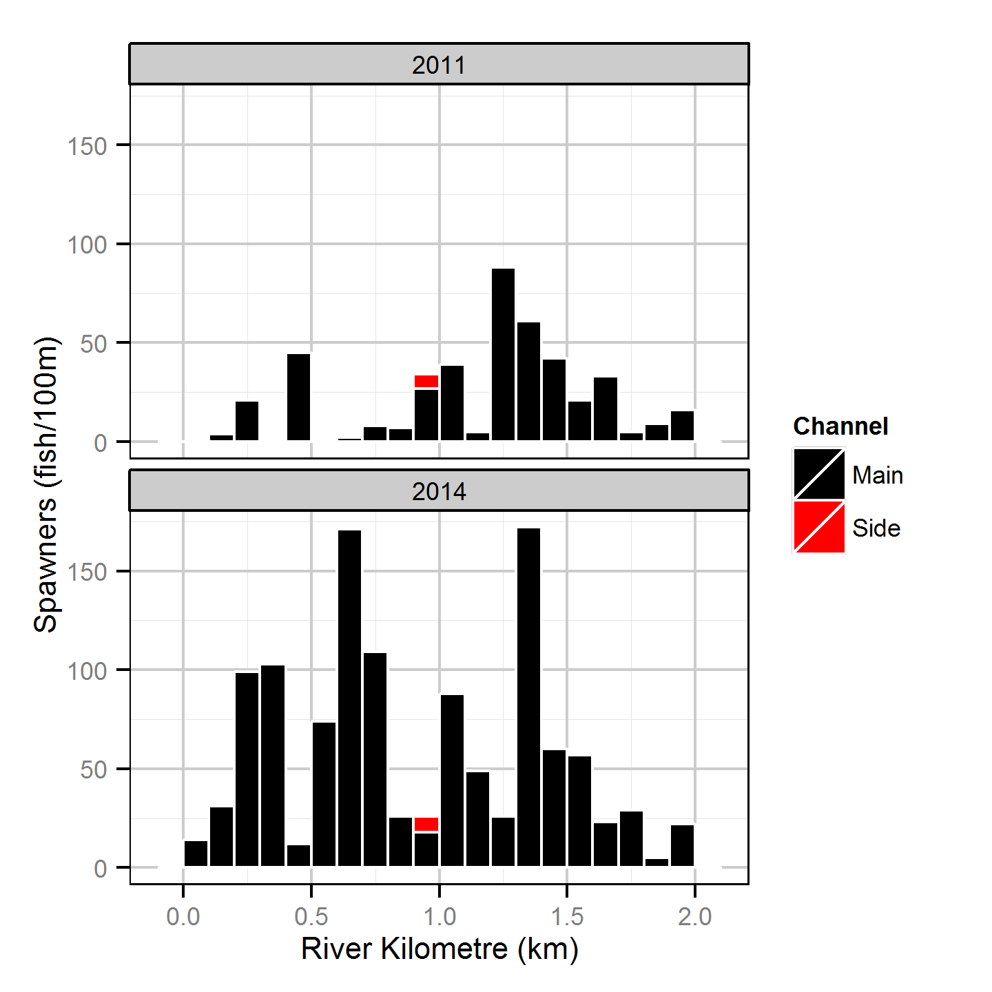
Norns Creek
References
M. J. Bradford, J. Korman and P. S. Higgins. “Using confidence intervals to estimate the response of salmon populations (Oncorhynchus spp.) to experimental habitat alterations”. In: Canadian Journal of Fisheries and Aquatic Sciences 62.12 (2005), pp. 2716-2726. ISSN: 0706-652X, 1205-7533. DOI: 10.1139/f05-179. <URL: http://www.nrcresearchpress.com/doi/abs/10.1139/f05-179> (visited on 07/07/2012).
M. Kéry and M. Schaub. Bayesian population analysis using WinBUGS : a hierarchical perspective. Boston: Academic Press, 2011. ISBN: 9780123870209 0123870208. <URL: http://www.vogelwarte.ch/bpa.html>.
C. J. Krebs. Ecological methodology. 2nd ed. Menlo Park, Calif: Benjamin/Cummings, 1999. ISBN: 0321021738.
M. Plummer. JAGS version 3.3.0 user manual. Oct. 2012. <URL: http://sourceforge.net/projects/mcmc-jags/files/Manuals/3.x/>.
R. C. Team. R: a language and environment for statistical computing. Vienna, Austria, 2013. <URL: http://www.R-project.org>.
Acknowledgements
The organisations and individuals whose contributions have made this analysis report possible include:
- BC Hydro
- Margo Dennis
- Guy Martel
- Philip Bradshaw
- James Baxter
- Mountain Water Research
- Jeremy Baxter
- Poisson Consulting
- Robyn Irvine
- Highland Helicopters
- Phil Hocking
- Mark Homis
- Golder Associates
- Dustin Ford
- Demitria Burgoon
- David Roscoe
- Additional Support
- Clint Tarala
- Gerry Nellestijn
- Gary Pavan
- Jay Bowers