Lower Columbia River Rainbow Trout Spawning Analysis 2015
The suggested citation for this analytic report is:
Thorley, J.L. and Hogan, P.M. (2016) Lower Columbia River Rainbow Trout Spawning Analysis 2015. A Poisson Consulting Analysis Report. URL: https://www.poissonconsulting.ca/f/1611032936.
Background
Each spring in the Lower Columbia River (LCR) below the Hugh L. Keenleyside Dam (HLK) and in the Lower Kootenay River (LKR) below the Brilliant Dam, thousands of Rainbow Trout spawn. Since 1992, BC Hydro has stabilized the spring discharge releases from HLK to protect Rainbow Trout redds from dewatering.
The primary goal of the current analysis to answer the following management questions:
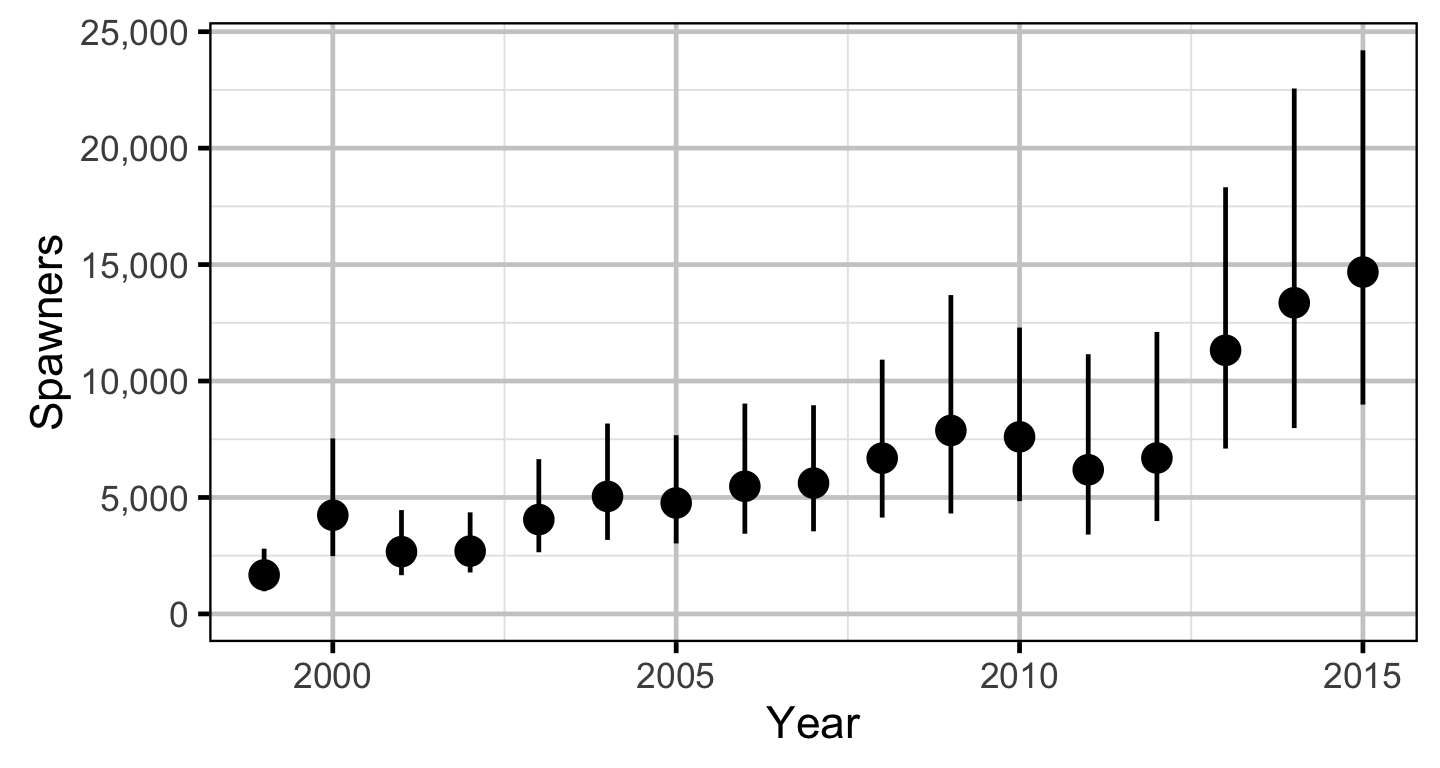
Does the implementation of Rainbow Trout Spawning Protection Flows over the course of the monitoring period lead to an increase in the relative abundance of Rainbow Trout spawning in the LCR downstream of the HLK dam?
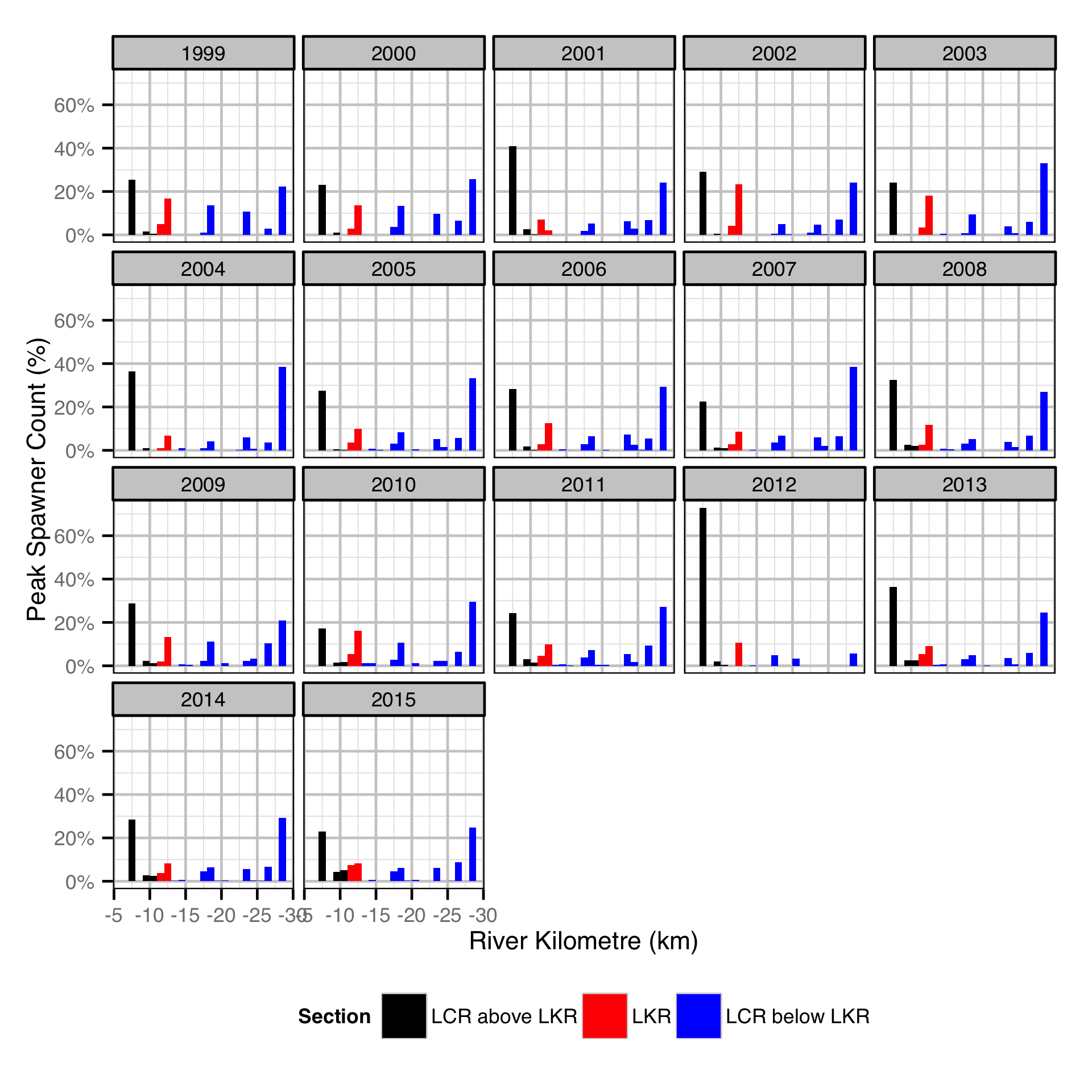
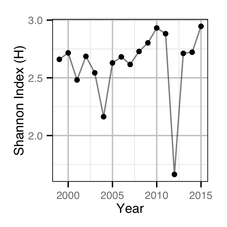
Does the implementation of RTSPF over the course of the monitoring period lead to an increase in the spatial distribution of locations (and associated habitat area) that Rainbow Trout use for spawning in the LCR downstream of HLK?
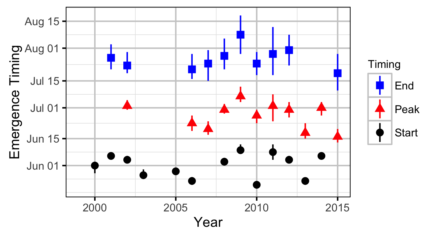
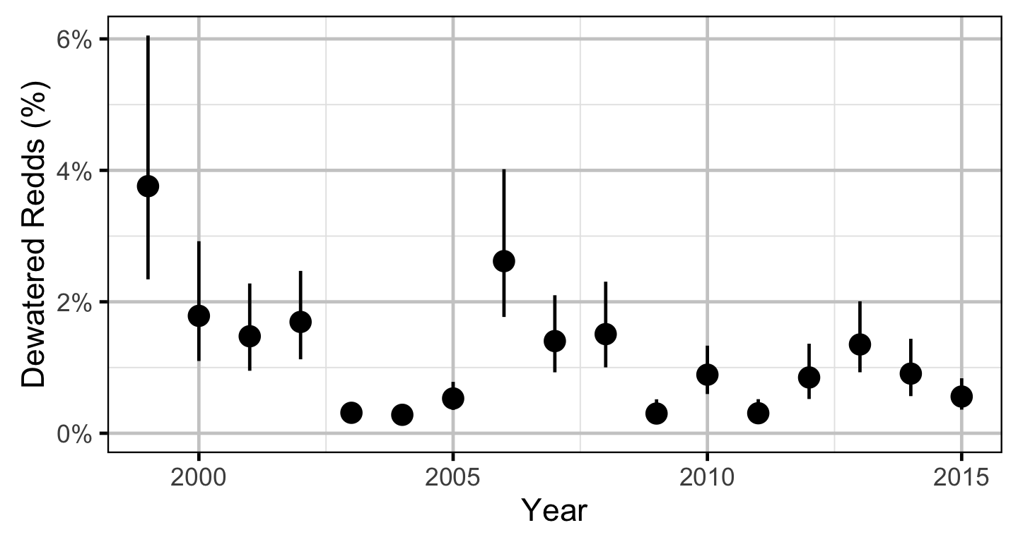
Does the implementation of RTSPF over the course of the monitoring period protect the majority of Rainbow Trout redds (as estimated from spawning timing) from being dewatered in the LCR downstream of HLK?
Methods
Data Preparation
The Rainbow Trout fish and redd aerial count data for the LCR and LKR were collected by Mountain Water Research and databased by Gary Pavan. The age-1 Rainbow Trout abundance data were provided by the Fish Population Indexing Program which is led by Golder Associates.
The study area was divided into three sections: the LCR above the LKR, the LKR and the LCR below the LKR. Redd and spawner counts upstream of Norns Creek Fan and downstream of Genelle were excluded from the section totals because they constitute less than 0.1% of the total count and were not surveyed in all years. The redd and spawner counts for the Right Upstream Bank above Robson Bridge were also excluded as they appear to be primarily driven by viewing conditions (and constitute less than 2.5% of the total). A decline in the redd count of more than one third of the previous maximum count for a particular section was inferred to be caused by poor viewing conditions (turbidity) and the affected spawner and redd section counts were excluded from any subsequent analyses.
Statistical Analysis
Hierarchical Bayesian models were fitted to the data using R version 3.2.3 (Team 2013) and JAGS 3.4.0 (Plummer 2012) which interfaced with each other via jaggernaut 2.3.1 (Thorley 2013). For additional information on hierarchical Bayesian modelling in the BUGS language, of which JAGS uses a dialect, the reader is referred to Kery and Schaub (2011, 41–44).
Unless indicated otherwise, the models used prior distributions that were vague in the sense that they did not affect the posterior distributions (Kery and Schaub 2011, 36). The posterior distributions were estimated from a minimum of 1,000 Markov Chain Monte Carlo (MCMC) samples thinned from the second halves of three chains (Kery and Schaub 2011, 38–40). Model convergence was confirmed by ensuring that Rhat (Kery and Schaub 2011, 40) was less than 1.1 for each of the parameters in the model (Kery and Schaub 2011, 61).
The posterior distributions of the fixed (Kery and Schaub 2011, 75) parameters are summarised in terms of a point estimate (mean), lower and upper 95% credible limits (2.5th and 97.5th percentiles), the standard deviation (SD), percent relative error (half the 95% credible interval as a percent of the point estimate) and significance (Kery and Schaub 2011, 37, 42).
Variable selection was achieved by dropping insignificant (Kery and Schaub 2011, 37, 42) fixed (Kery and Schaub 2011, 77–82) variables and uninformative random variables. A fixed variables was considered to be insignificant if its significance was \(\geq\) 0.05 while a random variable was considered to be uninformative if its percent relative error was \(\geq\) 80%. The Deviance Information Criterion (DIC) was not used because it is of questionable validity when applied to hierarchical models (Kery and Schaub 2011, 469).
The results are displayed graphically by plotting the modeled relationships between particular variables and the response with 95% credible intervals (CRIs) with the remaining variables held constant. In general, continuous and discrete fixed variables are held constant at their mean and first level values respectively while random variables are held constant at their typical values (expected values of the underlying hyperdistributions) (Kery and Schaub 2011, 77–82). Where informative the influence of particular variables is expressed in terms of the effect size (i.e., percent change in the response variable) with 95% CRIs (Bradford, Korman, and Higgins 2005).
Model Descriptions
The following model descriptions observe several conventions.
Acoustic Detection
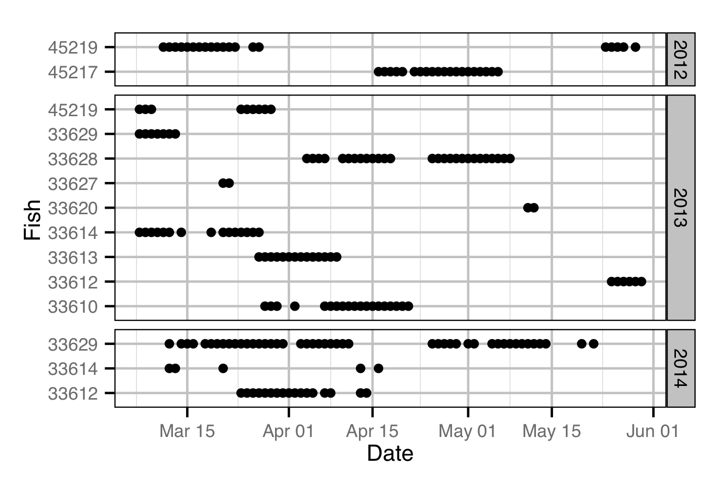
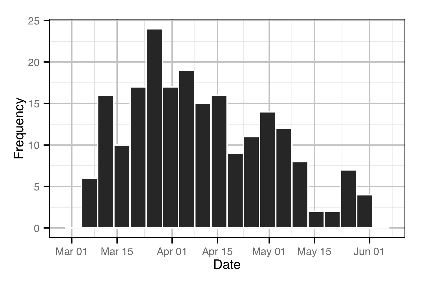
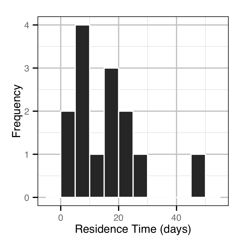
The spawner residence time in days at Norns Creek Fan was estimated from the acoustic detection data using a Generalised Linear Model. An acoustically tagged fish was considered to be resident on a particular day between March 7th and May 31st if it was detected by the Norns Creek receiver at location 1 for at least three hours (with at least three detections in each hour) between 8:00 and 12:00 (which corresponds to the general timing of the surveys).
Key assumptions of the residence time model include:
- The residual variation in spawner residence time is log-normally distributed.
Area-Under-The-Curve
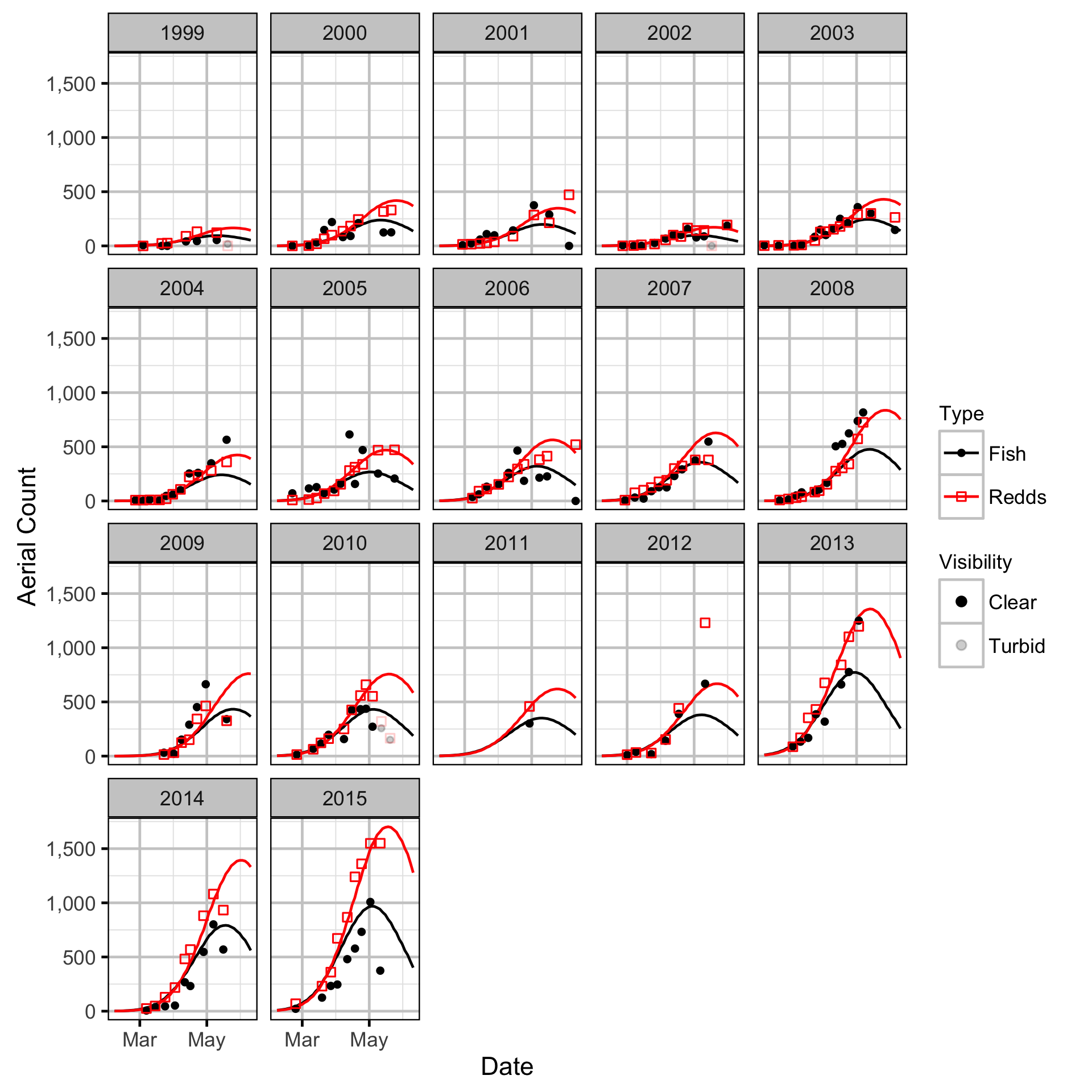
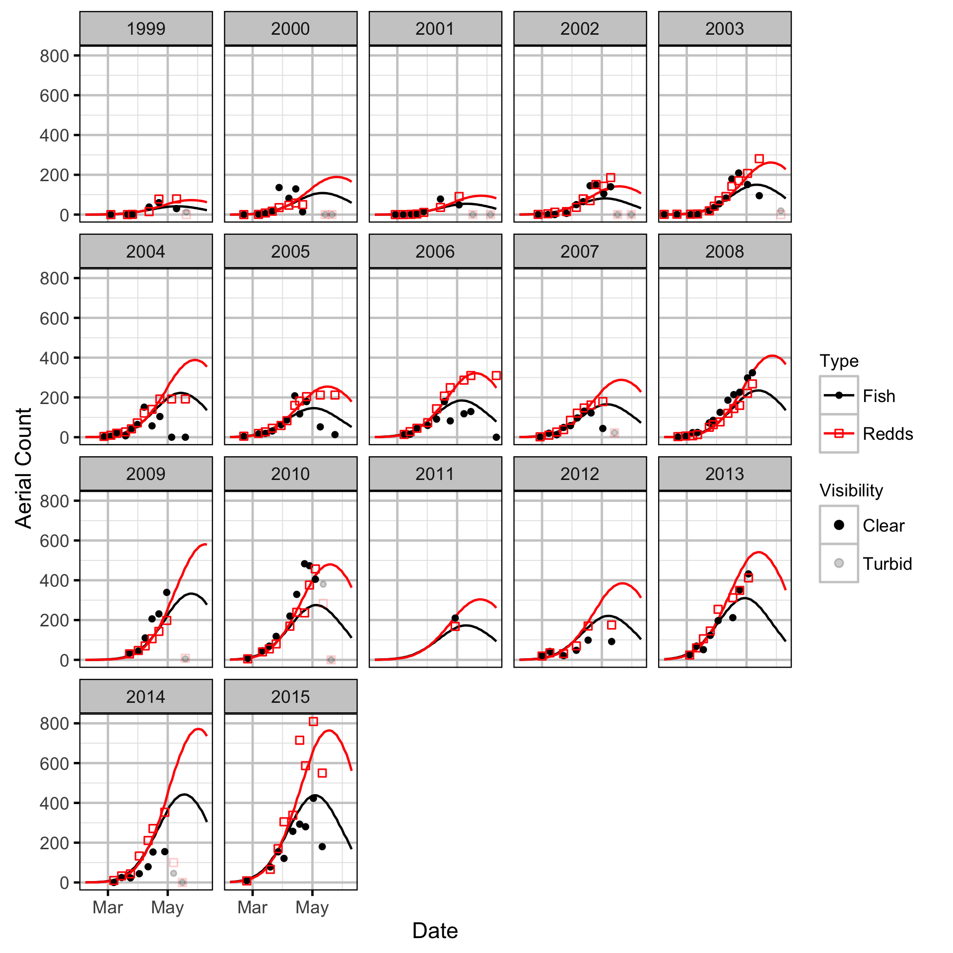
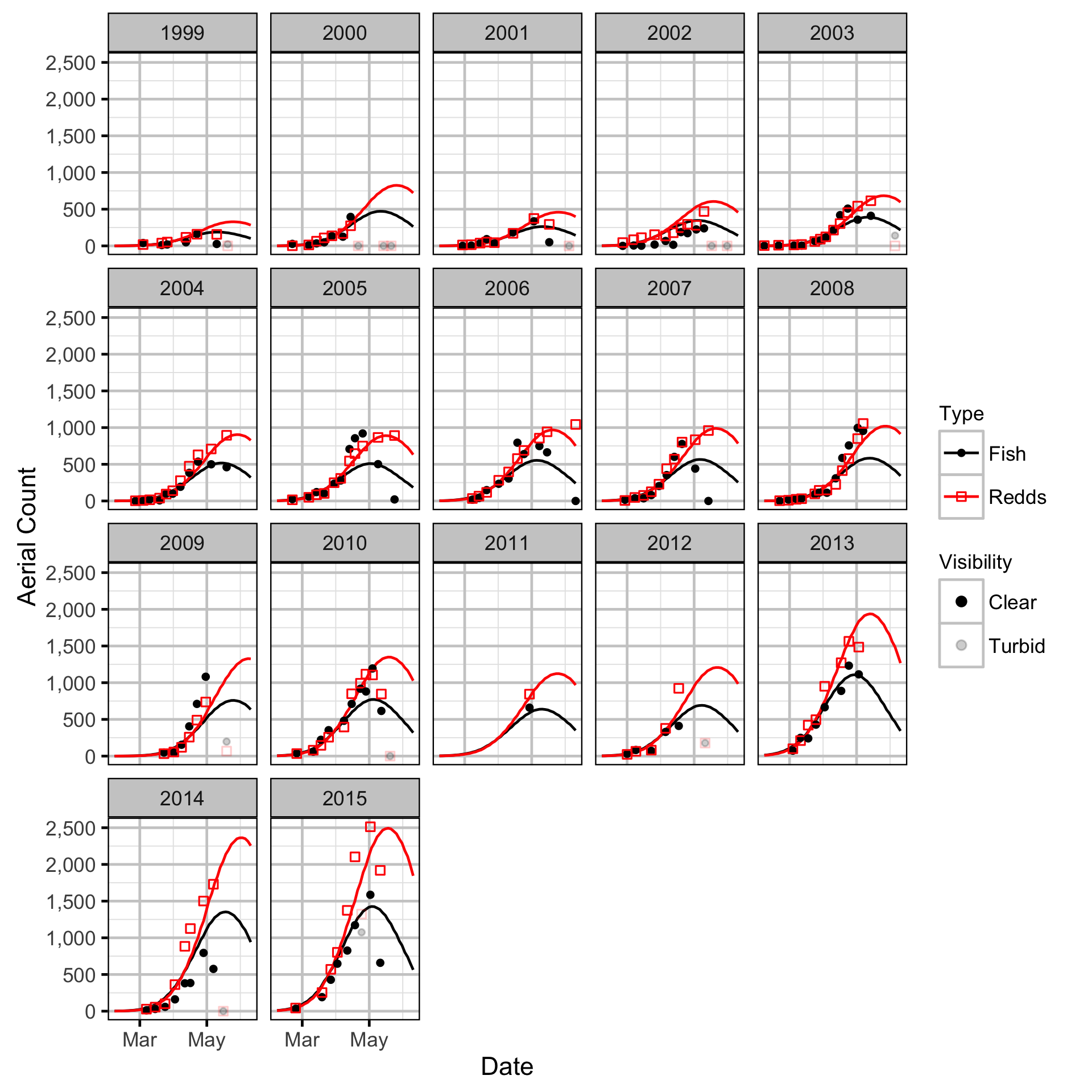
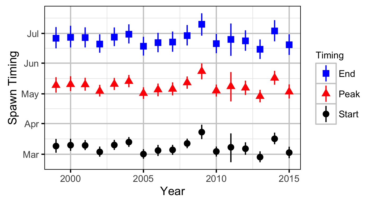
The spawner abundance and spawn timings were estimated from the aerial fish and redd counts for the three sections using an Area-Under-The-Curve (AUC) model.
Key assumptions of the AUC model include:
- Spawner and redd arrival and departure times are normally distributed.
- Spawner abundance varies by river section.
- Spawner abundance varies randomly by year and section within year.
- Spawner observer efficiency is between 0.9 and 1.1.
- Peak spawn timing varies randomly by year.
- Spawning duration varies by river section.
- Mean spawner residence time is as determined by the Acoustic Detection model.
- Redd observer efficiency is between 0.9 and 1.1.
- The number of redds per spawner is a fixed constant.
- The residual variations in the spawner and redd counts are described by separate overdispersed Poisson distributions.
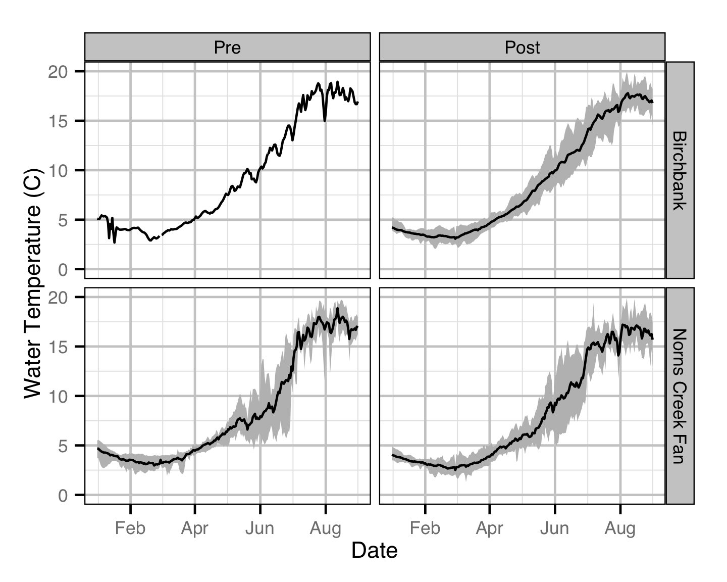
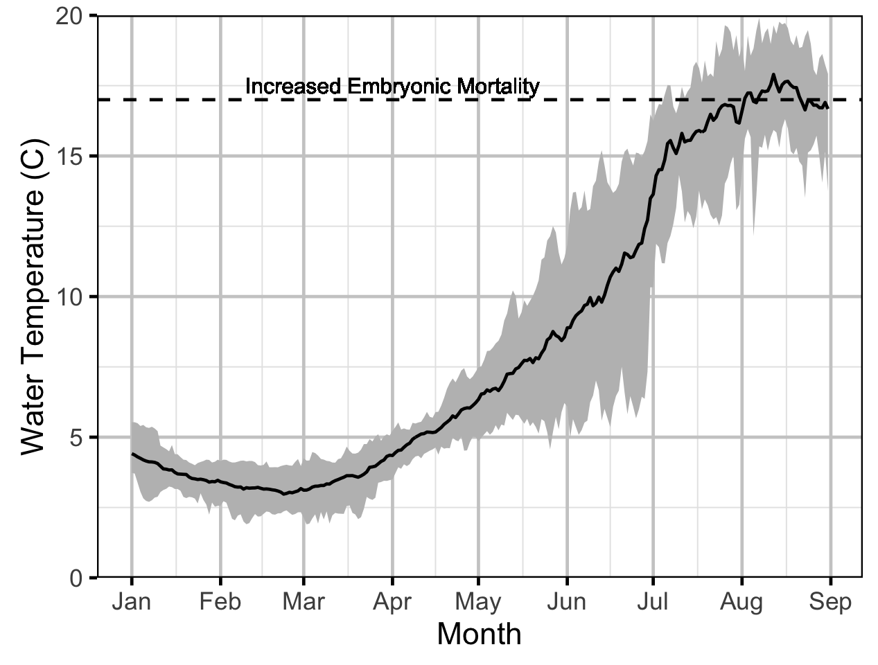
The expected emergence timing was calculated from the estimated spawn timing and the surface water temperature under the assumption that Rainbow Trout embryos emerge after 480 accumulated thermal units (ATUs).
The proportions of spawners at each site were used to calculate the Shannon Index, an information-theoretic measure of the diversity in the abundance distribution of a resource (Krebs 1999). In the current context, the Shannon Index takes into account both the number of spawning sites and how the spawning activity is distributed among these, with a higher index indicating a greater spatial distribution of spawning.
The Shannon Index \(H\) is given by \[ H = - \sum{p_i log(p_i)}\] where \(p_i\) is the proportion of the spawning activity at the \(i\)th location.
Stock-Recruitment
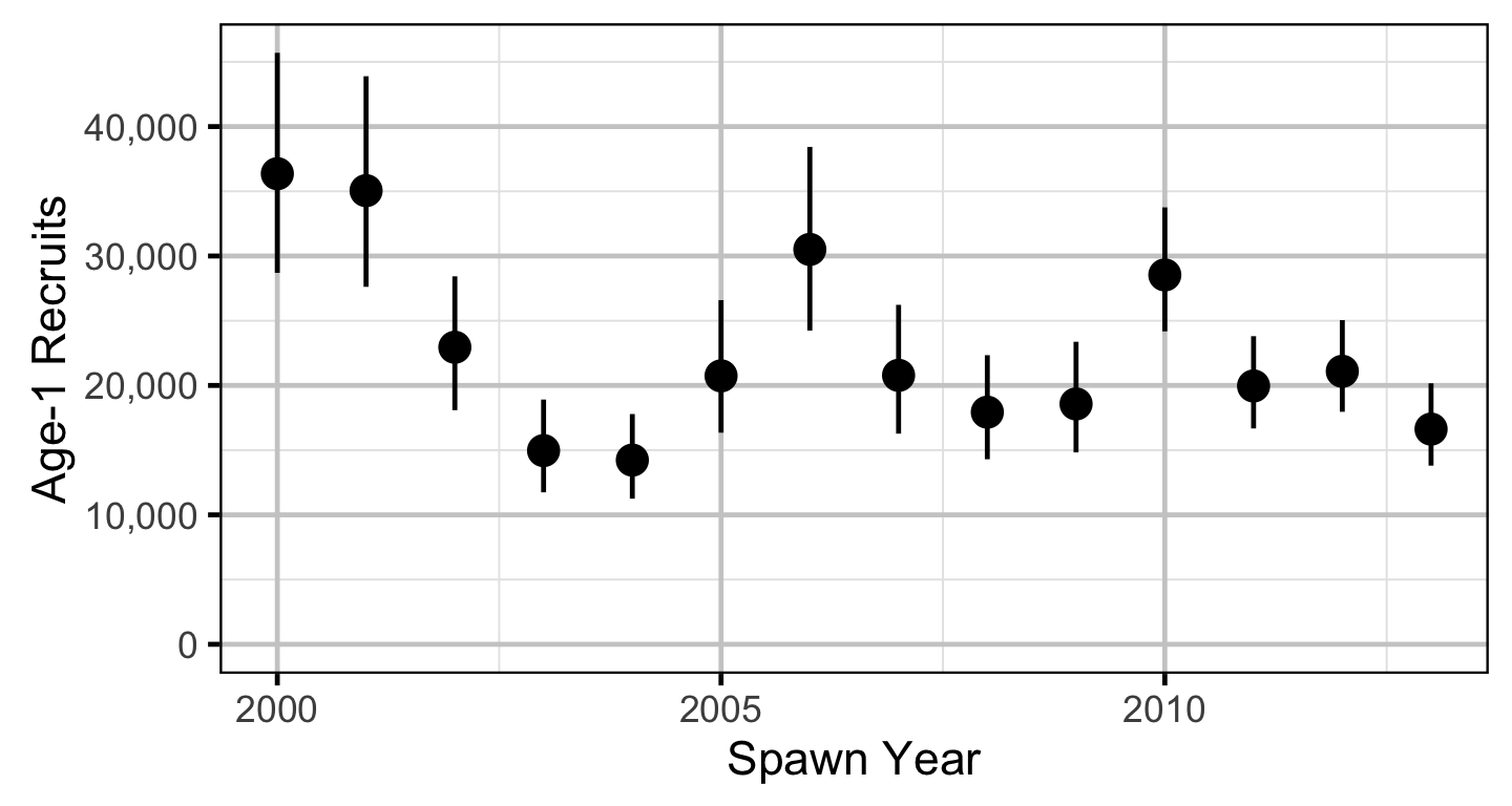
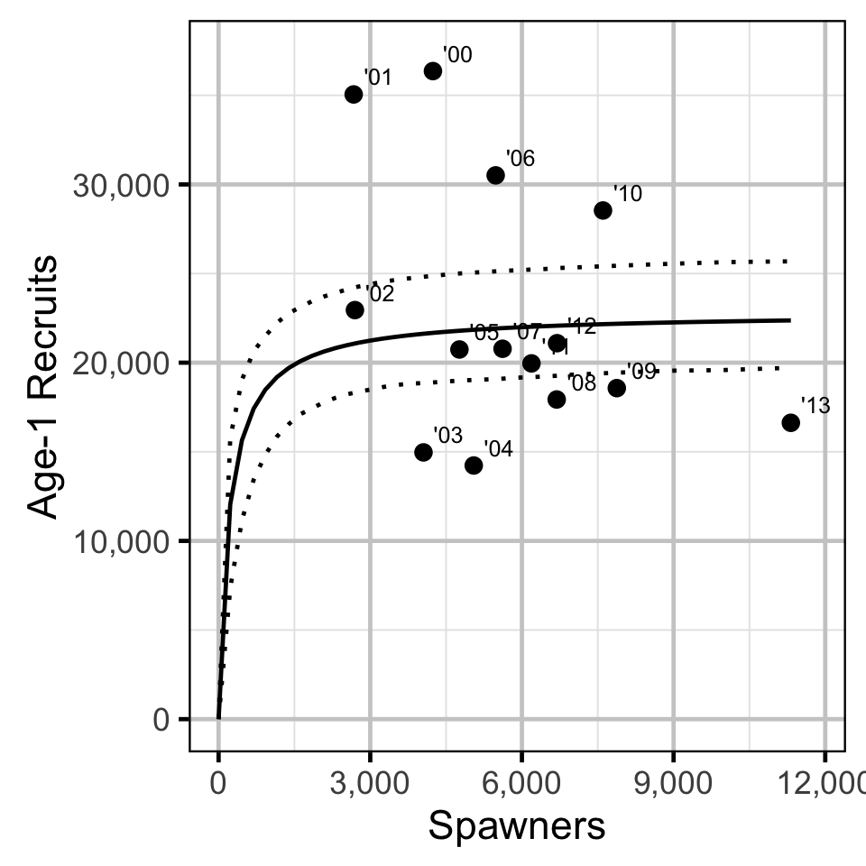
The relationship between the number of spawners and the number of age-1 recruits in the fall of the following year was estimated using a Beverton-Holt stock-recruitment model.
Key assumptions of the stock-recruitment model include:
- The prior probability distribution for the maximum number of recruits per spawner (
R0) is normally distributed with a mean of 90 and a SD of 50. - The residual variation in the number of age-1 recruits is log-normally distributed.
The prior probability distribution mean of 90 for R0 was based on an average of 2,900 eggs per female spawner, a 50:50 sex ratio, 50% egg survival, 50% post-emergence fall survival, 50% overwintering survival and 50% summer survival.
Model Code
The JAGS model code, which uses a series of naming conventions, is presented below.
Acoustic Detections
| Variable/Parameter | Description |
|---|---|
bResidenceTime |
Intercept of log(eResidenceTime) |
eResidenceTime[i] |
Expected residence time of ith spawner |
ResidenceTime[i] |
Observed residence time of ith spawner |
sResidenceTime |
SD of residual variation about log(eResidenceTime) |
Acoustic Detections - Model1
model{
  bResidenceTime ~ dnorm(0, 5^-2)
  sResidenceTime ~ dunif(0, 5)

  for(i in 1:length(ResidenceTime)){
    log(eResidenceTime[i]) <- bResidenceTime
    ResidenceTime[i] ~ dlnorm(log(eResidenceTime[i]), sResidenceTime^-2)
  }
}
Area-Under-The-Curve
| Variable/Parameter | Description |
|---|---|
bRdObsEfficiency |
Redd observer efficiency |
bRdResidence |
Redd residence time |
bReddPerSpawner |
Number of redds per spawner |
bSpAbundance |
Intercept of log(eSpAbundance) |
bSpAbundanceSite[i] |
Effect of ith site on log(eSpAbundance) |
bSpAbundanceSiteYear[i, j] |
Effect of ith site within jth year on log(eSpAbundance) |
bSpAbundanceYear[i] |
Effect of ith year on log(eSpAbundance) |
bSpArrivalPeak |
Intercept of eSpArrivalPeak |
bSpArrivalPeakYear[i] |
Effect of ith year on eSpArrivalPeak |
bSpArrivalWidthSite[i] |
Effect of ith site on log(eSpArrivalWidth) |
bSpObsEfficiency |
Spawner observer efficiency |
bSpResidence |
Spawner residence time |
Dayte[i] |
Day of the year on ith count |
eFishDispersion |
Overdispersion of Fish |
eRdAbundance[i] |
Expected redd abundance on ith count |
eReddDispersion |
Overdispersion of Redds |
eSpAbundance[i] |
Expected spawner abundance on ith count |
eSpArrivalPeak[i] |
Expected peak of spawner arrival timing on ith count |
eSpArrivalWidth[i] |
Expected SD of spawner arrival timing on ith count |
Fish[i] |
Observed number of fish on ith count |
Redds[i] |
Observed number of redds on ith count |
sFishDispersion |
SD of overdispersion for Fish |
Site[i] |
Site of ith count |
sReddDispersion |
SD of overdispersion for Redds |
sSpAbundanceSiteYear |
SD of effect of site within year on log(eSpAbundance) |
sSpAbundanceYear |
SD of effect of year on log(eSpAbundance) |
sSpArrivalPeakYear |
SD of effect of year on eSpArrivalPeak |
sSpArrivalWidth |
Intercept of log(eSpArrivalWidth) |
Year[i] |
Year of ith count |
Area-Under-The-Curve - Model1
model{
  bSpAbundance ~ dnorm(5, 5^-2)

  bSpArrivalPeak ~ dnorm(0, 14^-2)
  sSpArrivalWidth ~ dunif(log(14), log(42))
  bSpResidence ~ dnorm(11, 3.07^-2) T(6.31, 18.16)

  bSpObsEfficiency ~ dunif(0.9, 1.1)

  bSpAbundanceSite[1] <- 0
  for (i in 2:nSite) {
    bSpAbundanceSite[i] ~ dnorm(0, 2^-2)
  }

  sSpAbundanceYear ~ dunif(0, 2)
  for (i in 1:nYear) {
    bSpAbundanceYear[i] ~ dnorm(0, sSpAbundanceYear^-2)
  }

  sSpAbundanceSiteYear ~ dunif(0, 2)
  for (i in 1:nSite) {
    for (j in 1:nYear) {
      bSpAbundanceSiteYear[i, j] ~ dnorm(0, sSpAbundanceSiteYear^-2)
    }
  }

  sSpArrivalPeakYear ~ dunif(0, 28)
  for (i in 1:nYear) {
    bSpArrivalPeakYear[i] ~ dnorm(0, sSpArrivalPeakYear^-2)
  }

  bSpArrivalWidthSite[1] <- 0
  for(i in 2:nSite){
    bSpArrivalWidthSite[i] ~ dnorm(0, 1^-2)
  }

  bReddPerSpawner ~ dunif(0, 4)

  bRdResidence ~ dnorm(100, 50^-2)

  bRdObsEfficiency ~ dunif(0.9, 1.1)

  sFishDispersion ~ dunif(0, 2)
  sReddDispersion ~ dunif(0, 2)

  for (i in 1:length(Fish)) {
    log(eSpAbundance[i]) <- bSpAbundance +
                            bSpAbundanceSite[Site[i]] +
                            bSpAbundanceYear[Year[i]] +
                            bSpAbundanceSiteYear[Site[i], Year[i]]

    eSpArrivalPeak[i] <- bSpArrivalPeak + bSpArrivalPeakYear[Year[i]]
    log(eSpArrivalWidth[i]) <- sSpArrivalWidth + bSpArrivalWidthSite[Site[i]]

    eSpFracArrived[i] <- pnorm(
                           Dayte[i],
                           (eSpArrivalPeak[i] - bSpResidence/2),
                           eSpArrivalWidth[i]^-2
                         )
    eSpFracDeparted[i] <- pnorm(
                            Dayte[i],
                            (eSpArrivalPeak[i] + bSpResidence/2),
                            eSpArrivalWidth[i]^-2
                          )
    eFish[i] <- (eSpFracArrived[i] - eSpFracDeparted[i])
                * eSpAbundance[i]
                * bSpObsEfficiency

    eFishDispersion[i] ~ dgamma(1/sFishDispersion^2, 1/sFishDispersion^2)
    Fish[i] ~ dpois(eFish[i] * eFishDispersion[i])

    eRdAbundance[i] <- eSpAbundance[i] * bReddPerSpawner

    eRdFracArrived[i] <- pnorm(
                           Dayte[i],
                           (eSpArrivalPeak[i] - bSpResidence/2),
                           eSpArrivalWidth[i]^-2
                         )
    eRdFracDeparted[i] <- pnorm(
                            Dayte[i],
                            (eSpArrivalPeak[i] + bRdResidence/2),
                            eSpArrivalWidth[i]^-2
                          )
    eRedds[i] <- (eRdFracArrived[i] - eRdFracDeparted[i])
                 * eRdAbundance[i]
                 * bRdObsEfficiency

    eReddDispersion[i] ~ dgamma(1/sReddDispersion^2, 1/sReddDispersion^2)
    Redds[i] ~ dpois(eRedds[i] * eReddDispersion[i])
  }
}
Stock-Recruitment
| Variable/Parameter | Description |
|---|---|
eRecruits[i] |
Expected number of recruits in ith year |
k |
Maximum number of recruits |
R0 |
Maximum number of recruits per spawner |
Recruits[i] |
Observed number of age-1 fish in (i+1)th year |
sRecruits |
SD of residual variation about log(eRecruits) |
Stock[i] |
Observed number of spawners in ith year |
Stock-Recruitment - Model1
model{
  R0 ~ dnorm(90, 50^-2) T(0, )
  k ~  dnorm(2*10^4, (2*10^3)^-2) T(0, )
  sRecruits ~ dunif(0, 5)

  for(i in 1:length(Stock)){
    eRecruits[i] <- R0 * Stock[i] / (1 + Stock[i] * (R0 - 1) / k)
    Recruits[i] ~ dlnorm(log(eRecruits[i]), sRecruits^-2)
  }
}
Results
Model Parameters
The posterior distributions for the fixed (Kery and Schaub 2011 p. 75) parameters in each model are summarised below.
Acoustic Detections
| Parameter | Estimate | Lower | Upper | SD | Error | Significance |
|---|---|---|---|---|---|---|
| bResidenceTime | 2.3470 | 1.7430 | 2.9140 | 0.294 | 25 | 7e-04 |
| sResidenceTime | 1.0443 | 0.7157 | 1.6373 | 0.236 | 44 | 7e-04 |
| Convergence | Iterations |
|---|---|
| 1.01 | 1000 |
Area-Under-The-Curve
| Parameter | Estimate | Lower | Upper | SD | Error | Significance |
|---|---|---|---|---|---|---|
| bRdObsEfficiency | 0.99260 | 0.90380 | 1.09400 | 0.05670 | 10 | 0.0010 |
| bRdResidence | 71.01000 | 43.24000 | 110.14000 | 17.20000 | 47 | 0.0010 |
| bReddPerSpawner | 0.64620 | 0.46950 | 0.81150 | 0.08750 | 26 | 0.0010 |
| bSpAbundance | 7.41400 | 6.89100 | 7.98600 | 0.28100 | 7 | 0.0010 |
| bSpAbundanceSite[2] | -0.67200 | -0.84640 | -0.50110 | 0.08870 | 26 | 0.0010 |
| bSpAbundanceSite[3] | 0.53040 | 0.36200 | 0.70570 | 0.08810 | 32 | 0.0010 |
| bSpArrivalPeak | 33.99000 | 28.41000 | 40.10000 | 3.09000 | 17 | 0.0010 |
| bSpArrivalWidthSite[2] | -0.04748 | -0.08543 | -0.01241 | 0.01930 | 77 | 0.0119 |
| bSpArrivalWidthSite[3] | -0.02968 | -0.06604 | 0.00506 | 0.01867 | 120 | 0.1089 |
| bSpObsEfficiency | 1.00210 | 0.90600 | 1.09520 | 0.05760 | 9 | 0.0010 |
| bSpResidence | 13.93500 | 9.09600 | 17.87100 | 2.34800 | 31 | 0.0010 |
| sFishDispersion | 0.75820 | 0.70570 | 0.81970 | 0.02870 | 8 | 0.0010 |
| sReddDispersion | 0.29901 | 0.26981 | 0.32930 | 0.01520 | 10 | 0.0010 |
| sSpAbundanceSiteYear | 0.21160 | 0.14940 | 0.29320 | 0.03560 | 34 | 0.0010 |
| sSpAbundanceYear | 0.67090 | 0.45030 | 0.98870 | 0.14160 | 40 | 0.0010 |
| sSpArrivalPeakYear | 7.30400 | 4.60500 | 10.85600 | 1.66300 | 43 | 0.0010 |
| sSpArrivalWidth | 3.32390 | 3.26020 | 3.38670 | 0.03170 | 2 | 0.0010 |
| Convergence | Iterations |
|---|---|
| 1.16 | 8e+05 |
Stock-Recruitment
| Parameter | Estimate | Lower | Upper | SD | Error | Significance |
|---|---|---|---|---|---|---|
| k | 21239.0000 | 18616.0000 | 24129.0000 | 1426.0000 | 13 | 0.001 |
| R0 | 113.1000 | 42.6000 | 199.7000 | 42.0000 | 69 | 0.001 |
| sRecruits | 0.3406 | 0.2304 | 0.5183 | 0.0763 | 42 | 0.001 |
| Convergence | Iterations |
|---|---|
| 1.04 | 10000 |
Figures
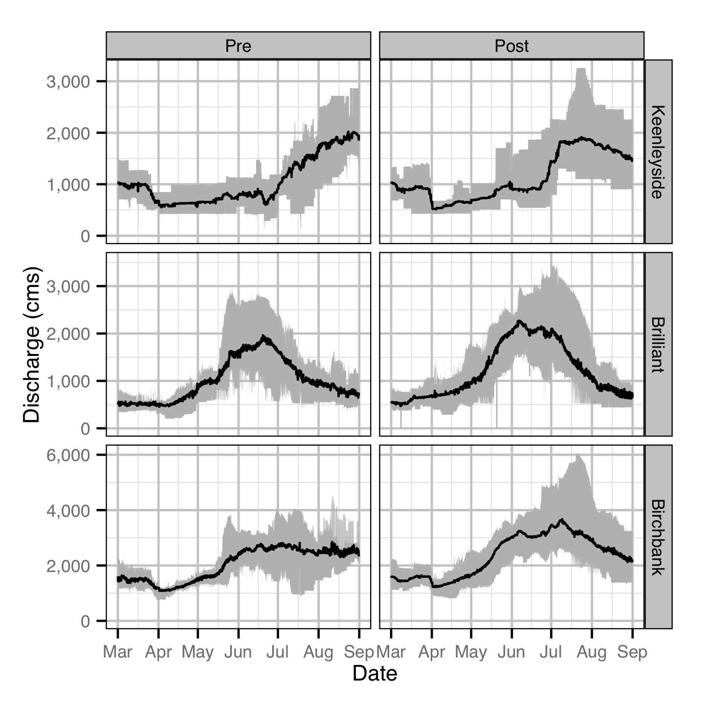
Discharge
Temperature
Acoustic Detections
Area-Under-The-Curve
Stock-Recruitment
Acknowledgements
The organisations and individuals whose contributions have made this analysis report possible include:
- BC Hydro
- Margo Dennis
- Guy Martel
- Philip Bradshaw
- James Baxter
- Mountain Water Research
- Jeremy Baxter
- Poisson Consulting
- Robyn Irvine
- Highland Helicopters
- Phil Hocking
- Mark Homis
- Golder Associates
- Dustin Ford
- Demitria Burgoon
- David Roscoe
- Additional Support
- Clint Tarala
- Gerry Nellestijn
- Gary Pavan
- Jay Bowers
References
Bradford, Michael J, Josh Korman, and Paul S Higgins. 2005. “Using Confidence Intervals to Estimate the Response of Salmon Populations (Oncorhynchus Spp.) to Experimental Habitat Alterations.” Canadian Journal of Fisheries and Aquatic Sciences 62 (12): 2716–26. https://doi.org/10.1139/f05-179.
Kery, Marc, and Michael Schaub. 2011. Bayesian Population Analysis Using WinBUGS : A Hierarchical Perspective. Boston: Academic Press. http://www.vogelwarte.ch/bpa.html.
Krebs, Charles J. 1999. Ecological Methodology. 2nd ed. Menlo Park, Calif: Benjamin/Cummings.
Plummer, Martyn. 2012. “JAGS Version 3.3.0 User Manual.” http://sourceforge.net/projects/mcmc-jags/files/Manuals/3.x/.
Team, R Core. 2013. “R: A Language and Environment for Statistical Computing.” Vienna, Austria: R Foundation for Statistical Computing. http://www.R-project.org.
Thorley, J. L. 2013. “Jaggernaut: An R Package to Facilitate Bayesian Analyses Using JAGS (Just Another Gibbs Sampler).” Nelson, B.C.: Poisson Consulting Ltd. https://github.com/poissonconsulting/jaggernaut.