Lower Columbia River Rainbow Trout Spawning 2020
The suggested citation for this analytic appendix is:
Thorley, J.L. and Amies-Galonski, E. (2021) Lower Columbia River Rainbow Trout Spawning 2020. A Poisson Consulting Analytic Appendix. URL: https://www.poissonconsulting.ca/f/626789785.
Background
Each spring in the Lower Columbia River (LCR) below Hugh L. Keenleyside Dam (HLK) and in the Lower Kootenay River (LKR) below Brilliant Dam, thousands of Rainbow Trout spawn.
Since 1992, BC Hydro has stabilized the spring discharge releases from HLK to protect Rainbow Trout redds from dewatering.
The primary goal of the current analysis to estimate the abundance of spawners, egg survival and the stock-recruitment relationship. We also explore the use of drone imagery for redd mapping.
Data Preparation
The aerial spawner counts were conducted by Mountain Water Research. The age-1 recruitment estimates were provided by the Fish Population Indexing Program. The drone surveys were conducted by Harrier Aerial Surveys. The remaining data were collected by Mountain Water Research, Poisson Consulting and Nuupqu.
The study area was divided into seven sections: Norns Creek Fan (NCF), NCF to LKR, LKR, LKR to Genelle, Genelle. Redd and spawner counts upstream of Norns Creek Fan and downstream of Genelle were excluded from the section totals because they constitute less than 0.1% of the total count and were not surveyed in all years. The redd and spawner counts for the Right Upstream Bank above Robson Bridge were also excluded as they appear to be primarily driven by viewing conditions (and constitute less than 2.5% of the total). Viewing conditions were classified as Good or Poor. If information on the viewing conditions was not available a decline in the redd count of more than one third of the cumulative maximum count for a particular section was assumed to be caused by poor viewing conditions.
The mapped peak redd and fish counts are the peak counts for that site.
The data were prepared for analysis using R version 4.0.4 (R Core Team 2017).
Statistical Analysis
Model parameters were estimated using Bayesian methods. The estimates were produced using JAGS (Plummer 2015) and STAN (Carpenter et al. 2017). For additional information on Bayesian estimation the reader is referred to McElreath (2016).
Unless stated otherwise, the Bayesian analyses used weakly informative normal and half-normal prior distributions (Gelman, Simpson, and Betancourt 2017). The posterior distributions were estimated from 1500 Markov Chain Monte Carlo (MCMC) samples thinned from the second halves of 3 chains (Kery and Schaub 2011, 38–40). Model convergence was confirmed by ensuring that the potential scale reduction factor \(\hat{R} \leq 1.05\) (Kery and Schaub 2011, 40) and the effective sample size (Brooks et al. 2011) \(\textrm{ESS} \geq 150\) for each of the monitored parameters (Kery and Schaub 2011, 61).
The parameters are summarised in terms of the point estimate, standard deviation (sd), the z-score, lower and upper 95% confidence/credible limits (CLs) and the p-value (Kery and Schaub 2011, 37, 42). The estimate is the median (50th percentile) of the MCMC samples, the z-score is \(\mathrm{mean}/\mathrm{sd}\) and the 95% CLs are the 2.5th and 97.5th percentiles. A p-value of 0.05 indicates that the lower or upper 95% CL is 0.
The results are displayed graphically by plotting the modeled relationships between particular variables and the response(s) with the remaining variables held constant. In general, continuous and discrete fixed variables are held constant at their mean and first level values, respectively, while random variables are held constant at their typical values (expected values of the underlying hyperdistributions) (Kery and Schaub 2011, 77–82). When informative the influence of particular variables is expressed in terms of the effect size (i.e., percent change in the response variable) with 95% confidence/credible intervals (CIs, Bradford, Korman, and Higgins 2005).
The analyses were implemented using R version 4.0.4
(R Core Team 2019) and the
mbr family of packages.
Model Descriptions
Area-Under-The-Curve
The spawner abundance and spawn timings were estimated from the aerial fish and redd counts for the five sections (in three segments) using an Area-Under-The-Curve (AUC) model.
Key assumptions of the AUC model include:
- Spawner abundance varies by river section.
- Spawner abundance varies randomly by year and section within year.
- Spawner observer efficiency is between 0.8 and 1.0.
- Number of redds per spawner is between 1 and 2.
- Spawner residence time is between 14 and 21 days as determined in a previous year’s analysis.
- Redd residence time is between 30 and 40 days.
- Spawner arrival and departure times are normally distributed.
- Spawner arrival duration (SD of normal distribution) varies randomly by river segment.
- Peak spawner arrival timing varies randomly by year.
- The residual variations in the spawner and redd counts are described by separate Negative Binomial distributions.
Stock-Recruitment
The relationship between the number of spawners/eggs and the resultant number of age-1 fish was estimated using a Beverton-Holt stock-recruitment model (Walters and Martell 2004):
\[ R = \frac{\alpha \cdot S}{1 + \beta \cdot S}\]
where \(S\) is the stock (spawners or eggs), \(R\) is the recruits, \(\alpha\) is the recruits per stock at low density and \(\beta\) determines the density-dependence.
The carrying capacity is \(\alpha / \beta\).
Key assumptions of the stock-recruitment model include:
- The expected number of recruits varies with the proportion of redds dewatered.
- The residual variation in the number of recruits is log-normally distributed.
Spawners
Key assumptions of the spawner stock-recruitment model include:
- The recruits per spawner at low density (\(\alpha\)) is normally distributed with a mean of 90 and a SD of 50.
The mean of 90 for \(\alpha\) was based on an average of 2,900 eggs per female spawner, a 50:50 sex ratio, 50% egg survival, 50% post-emergence fall survival, 50% overwintering survival and 50% summer survival.
Eggs
Key assumptions of the egg stock-recruitment model include:
- The recruits per spawner at low density (\(\alpha\)) is normally distributed with a mean of 0.0625 and a SD of 0.03.
The mean of 0.625 is based on a 50% egg survival, 50% post-emergence fall survival, 50% overwintering survival and 50% summer survival.
Stage
The spreadsheet Norn's Fan stage discharge curve.xls predicts the
stage at CNN (in m) from the discharge (in cms) from HLK and BRDs dam
based on the multiple regression equation
\[\text{CNN} = 417.133 + 0.001883826 \cdot \text{HLK} + 0.000559058 \cdot \text{BRD}\]
We predict the stage from the discharge using a multiple second-order polynomial regression with interactions. The main part model was of the following form:
\[\text{CNN} = \text{b0} + \text{bHLK} \cdot \text{HLK} + \text{bHLK2} \cdot \text{HLK}^2 + \text{bBRD} \cdot \text{BRD} + \text{bBRD2} \cdot \text{BRD}^2 + \text{bHLKBRD} \cdot \text{HLK} \cdot \text{BRD} + \text{bHLK2BRD} \cdot \text{HLK}^2 \cdot \text{BRD}\] To ensure model convergence \(\text{HLK}\) and \(\text{BRD}\) were the standardized discharges. The model also included a parameter to correct for an offset in \(\text{CNN}\) from May 1st 2017.
Model Templates
Area-Under-The-Curve
data {
  int<lower=0> nObs;
  int<lower=0> nSection;
  int<lower=0> nSegment;
  int<lower=0> nYear;

  int Year[nObs];
  int Section[nObs];
  int Segment[nObs];
  real Doy[nObs];
  int Fish[nObs];
  int Redds[nObs];
parameters {
  vector<lower=3,upper=9>[nSection] bFishAbundanceSection;

  real<lower=0> sFishAbundanceYear;
  vector[nYear] bFishAbundanceYear;
  real<lower=0> sFishAbundanceSectionYear;
  vector[nSection * nYear] bFishAbundanceSectionYear;

  real<lower=0.8,upper=1.0> bFishObserverEfficiency;
  real<lower=0.0,upper=2.0> bReddObserverEfficiency;

  real<lower=1, upper=2> bReddPerFish;

  real<lower=14, upper=21> bFishResidenceTime;
  real<lower=30, upper=40> bReddResidenceTime;

  real<lower=100, upper=150> bPeakFishArrivalTiming;

  real<lower=0,upper=21> sPeakFishArrivalTimingYear;
  vector[nYear] bPeakFishArrivalTimingYear;

  real<lower=log(10), upper=log(50)> bFishArrivalDuration;

  real<lower=0> sFishArrivalDurationSegmentYear;
  vector[nSegment * nYear] bFishArrivalDurationSegmentYear;

  real<lower=0, upper=2> bDispersionRedds;
  real<lower=0, upper=2> bDispersionFish;
model {
  vector[nObs] eFishAbundance;
  vector[nObs] ePeakFishArrivalTiming;
  vector[nObs] eFishArrivalDuration;

  vector[nObs] eRedds;
  vector[nObs] eFish;

  sFishAbundanceYear ~ normal(0, 1);
  bFishAbundanceYear ~ normal(0, sFishAbundanceYear);
  sFishAbundanceSectionYear ~ normal(0, 1);
  bFishAbundanceSectionYear ~ normal(0, sFishAbundanceSectionYear);

  bPeakFishArrivalTimingYear ~ normal(0, sPeakFishArrivalTimingYear);
  bFishArrivalDurationSegmentYear ~ normal(0, 1);
  bFishArrivalDurationSegmentYear ~ normal(0, sFishArrivalDurationSegmentYear);

  for (i in 1:nObs) {
    eFishAbundance[i] = exp(bFishAbundanceSection[Section[i]] + bFishAbundanceYear[Year[i]] + bFishAbundanceSectionYear[((Section[i] - 1) * Year[i]) + Year[i]]);

    ePeakFishArrivalTiming[i] = bPeakFishArrivalTiming + bPeakFishArrivalTimingYear[Year[i]];

    eFishArrivalDuration[i] = exp(bFishArrivalDuration + bFishArrivalDurationSegmentYear[((Segment[i] - 1) * Year[i]) + Year[i]]);

    eRedds[i] = eFishAbundance[i] * bReddPerFish * bReddObserverEfficiency * (normal_cdf(Doy[i], ePeakFishArrivalTiming[i], eFishArrivalDuration[i]) - normal_cdf(Doy[i], ePeakFishArrivalTiming[i] + bReddResidenceTime, eFishArrivalDuration[i]));

    eFish[i] = eFishAbundance[i] * bFishObserverEfficiency * (normal_cdf(Doy[i], ePeakFishArrivalTiming[i], eFishArrivalDuration[i]) - normal_cdf(Doy[i], ePeakFishArrivalTiming[i] + bFishResidenceTime, eFishArrivalDuration[i]));
  }
  Redds ~ neg_binomial_2(eRedds, 1/bDispersionRedds);
  Fish ~ neg_binomial_2(eFish, 1/bDispersionFish);
Block 1. Model description.
Stock-Recruitment
Spawners
.model {

  bAlpha ~ dnorm(90, 50^-2) T(1,)
  bBeta ~ dnorm(0, 1/10^-2) T(0,)

  bDewatered ~ dnorm(0, 100^-2)

  sRecruits ~ dnorm(0, 2^-2) T(0, )
 for(i in 1:length(Stock)) {
    log(eRecruits[i]) <- log(bAlpha * Stock[i] / (1 + bBeta * Stock[i])) + bDewatered * Dewatered[i]
    Recruits[i] ~ dlnorm(log(eRecruits[i]), sRecruits^-2)
  }
Block 2. Model description.
Eggs
.model {
  bAlpha ~ dnorm(0.0625, 0.03^-2) T(0,)
  bBeta ~ dnorm(0, 1/100000^-2) T(0, )

  bEggLoss ~ dnorm(0, 100^-2)

  sRecruits ~ dnorm(0, 2^-2) T(0,)
  for(i in 1:length(Recruits)){
    log(eRecruits[i]) <- log(bAlpha * Eggs[i] / (1 + bBeta * Eggs[i])) + bEggLoss * EggLoss[i]
    Recruits[i] ~ dlnorm(log(eRecruits[i]), sRecruits^-2)
  }
Block 3.
Stage
.model{
  bIntercept ~ dnorm(420, 2^-2)

  bOffset[1] <- 0
  for(i in 2:nOffset) {
    bOffset[i] ~ dnorm(0, 1^-2)
  }

  bHLK ~ dnorm(0, 1^-2)
  bHLK2 ~ dnorm(0, 1^-2)

  bLKR ~ dnorm(0, 1^-2)
  bLKR2 ~ dnorm(0, 1^-2)

  bHLKLKR ~ dnorm(0, 1^-2)
  bHLK2LKR ~ dnorm(0, 1^-2)

  bCor <- 0.4
  eCorStage[1] <- eStage[1]
  for(i in 2:length(Stage)){
    eCorStage[i] <- eStage[i] + bCor^(Days[i] - Days[i-1]) * (Stage[i-1] - eStage[i-1])
  }

  sStage ~ dnorm(0, 1^-2) T(0, )
  for(i in 1:length(Stage)){
    eStage[i] <- bIntercept + bOffset[Offset[i]] + bHLK * HLK[i] + bLKR * LKR[i] + bHLK2 * HLK[i]^2 + bLKR2 * LKR[i]^2 + bHLKLKR * HLK[i] * LKR[i] + bHLK2LKR * HLK[i]^2 * LKR[i]

    Stage[i] ~ dnorm(eCorStage[i], sStage^-2)
  }
Block 4. The model description.
Results
Tables
Dewatering
Table 1.
| ReductionDate | HLK_ALH_Start | HLK_ALH_End | BRD_BRDS_BRX_Start | BRD_BRDS_BRX_End | DewateredRedds | AerialSite |
|---|---|---|---|---|---|---|
| 2020-02-29 | 1096 | 701 | 898 | 897 | 6 | Norns Creek Fan |
| 2020-03-07 | 661 | 424 | 679 | 682 | 0 | Norns Creek Fan |
| 2020-03-31 | 1024 | 547 | 349 | 349 | 10 | Norns Creek Fan |
| 2020-03-31 | 1024 | 547 | 349 | 349 | 55 | Norns Creek Fan |
| 2020-03-31 | 1024 | 547 | 349 | 349 | 0 | Norns Creek Fan |
| 2020-05-09 | 900 | 723 | 1152 | 1155 | 0 | Norns Creek Fan |
| 2020-06-12 | 780 | 438 | 2304 | 2255 | 117 | Norns Creek Fan |
| 2020-03-31 | 1024 | 547 | 349 | 349 | 2 | RUB, Kinnaird |
| 2020-03-31 | 1024 | 547 | 349 | 349 | 0 | RUB, Kinnaird |
| 2020-05-09 | 900 | 723 | 1152 | 1155 | 0 | RUB, Kinnaird |
| 2020-05-09 | 900 | 723 | 1152 | 1155 | 0 | Oxbow (Total) |
| 2020-03-07 | 661 | 424 | 679 | 682 | 0 | Genelle (Total) |
| 2020-03-31 | 1024 | 547 | 349 | 349 | 0 | Genelle (Total) |
| 2020-03-31 | 1024 | 547 | 349 | 349 | 2 | Genelle (Total) |
| 2020-03-31 | 1024 | 547 | 349 | 349 | 0 | Genelle (Total) |
| 2020-05-09 | 900 | 723 | 1152 | 1155 | 0 | Genelle (Total) |
Area-Under-The-Curve
Table 2. Parameter descriptions.
| Parameter | Description |
|---|---|
bDispersionFish |
Clustering parameter for Fish |
bDispersionRedds |
Clustering parameter for Redds |
bFishAbundanceSection[i] |
Intercept for log(eFishAbundance) by
Section |
bFishAbundanceSectionYear[i] |
Effect of Section by Year on
bFishAbundanceSection |
bFishAbundanceYear[i] |
Effect of ith Year on
bFishAbundanceSection |
bFishArrivalDuration[i] |
Intercept for log(eFishArrivalDuration) |
bFishArrivalDurationSegmentYear[i] |
Effect of Segment by Year on
bFishArrivalDuration |
bFishObsEfficiency |
Fish observer efficiency |
bFishResidenceTime |
Fish residence time (days) |
bPeakFishArrivalTiming |
Intercept for ePeakFishArrivalTiming |
bPeakFishArrivalTimingYear[i] |
Effect of ith Year on
bPeakFishArrivalTiming |
bReddObserverEfficiency |
Redd observer efficiency |
bReddPerFish |
Number of Redds per Fish |
bReddResidenceTime |
Redd residence time (days) |
Doy[i] |
Day of the year of ith count |
eFishAbundance[i] |
Expected Fish abundance for ith count |
eFishArrivalDuration[i] |
Expected SD of Fish arrival timing for
ith count |
ePeakFishArrivalTiming[i] |
Expected Doy of peak Fish arrival for
ith count |
Fish[i] |
Observed number of Fish on ith count |
Redds[i] |
Observed number of Redds on ith count |
Section[i] |
Section of ith count |
Segment[i] |
Segment of ith count |
sFishAbundanceSectionYear |
SD of bFishAbundanceSectionYear |
sFishAbundanceYear |
SD of bFishAbundanceYear |
sFishArrivalDurationSegmentYear |
SD of bFishArrivalDurationSegmentYear |
sPeakFishArrivalTimingYear |
SD of bPeakFishArrivalTimingYear |
Year[i] |
Year of ith count |
Table 3. Model coefficients.
| term | estimate | sd | zscore | lower | upper | pvalue |
|---|---|---|---|---|---|---|
| bDispersionFish | 0.4881459 | 0.0263758 | 18.535762 | 0.4394182 | 0.5432272 | 0.0006662 |
| bDispersionRedds | 0.2044098 | 0.0133868 | 15.332096 | 0.1812775 | 0.2332868 | 0.0006662 |
| bFishAbundanceSection[1] | 4.6069291 | 0.2101128 | 21.905750 | 4.1572600 | 4.9966890 | 0.0006662 |
| bFishAbundanceSection[2] | 7.3143280 | 0.2056670 | 35.531545 | 6.8806470 | 7.6914124 | 0.0006662 |
| bFishAbundanceSection[3] | 6.6668701 | 0.2163050 | 30.832218 | 6.2312894 | 7.0844799 | 0.0006662 |
| bFishAbundanceSection[4] | 7.1982436 | 0.2145053 | 33.554745 | 6.7556643 | 7.6023303 | 0.0006662 |
| bFishAbundanceSection[5] | 7.1787053 | 0.2214169 | 32.483602 | 6.7373831 | 7.6137550 | 0.0006662 |
| bFishArrivalDuration | 3.1541295 | 0.0333211 | 94.629356 | 3.0852216 | 3.2162872 | 0.0006662 |
| bFishObserverEfficiency | 0.9060714 | 0.0564932 | 16.026254 | 0.8069395 | 0.9945786 | 0.0006662 |
| bFishResidenceTime | 19.6155834 | 1.3261666 | 14.588611 | 16.0567768 | 20.9577444 | 0.0006662 |
| bPeakFishArrivalTiming | 117.7365964 | 2.2804827 | 51.642642 | 113.4071356 | 122.3378574 | 0.0006662 |
| bReddObserverEfficiency | 0.6088296 | 0.1352292 | 4.590920 | 0.4106069 | 0.8901945 | 0.0006662 |
| bReddPerFish | 1.4030021 | 0.2915530 | 4.947118 | 1.0184286 | 1.9700875 | 0.0006662 |
| bReddResidenceTime | 31.6837346 | 1.7833351 | 18.037807 | 30.0753670 | 36.6927115 | 0.0006662 |
| sFishAbundanceSectionYear | 0.4201935 | 0.0488669 | 8.676054 | 0.3373028 | 0.5312576 | 0.0006662 |
| sFishAbundanceYear | 0.7843049 | 0.1393409 | 5.745200 | 0.5711731 | 1.1192612 | 0.0006662 |
| sFishArrivalDurationSegmentYear | 0.1671884 | 0.0245854 | 6.901190 | 0.1275677 | 0.2197261 | 0.0006662 |
| sPeakFishArrivalTimingYear | 7.9905815 | 1.6662814 | 4.938542 | 5.6100701 | 12.2189231 | 0.0006662 |
Table 4. Model summary.
| n | K | nchains | niters | nthin | ess | rhat | converged |
|---|---|---|---|---|---|---|---|
| 877 | 18 | 3 | 500 | 1 | 322 | 1.012 | TRUE |
Stock-Recruitment
Spawners
Table 5. Parameter descriptions.
| Parameter | Description |
|---|---|
bAlpha |
Intercept for eAlpha |
bBeta |
Intercept for log(eBeta) |
bDewatered |
Effect of Dewatered on log(bAlpha) |
Dewatered[i] |
Proportional redd dewatering in ith spawn year |
eAlpha |
Expected number of recruits at low density |
eBeta |
Expected density-dependence |
eRecruits[i] |
Expected Recruits |
Recruits[i] |
Number of age-1 recruits from ith spawn year |
sRecruits |
SD of residual variation in Recruits |
Stock[i] |
Number of spawners in ith spawn year |
Table 6. Model coefficients.
| term | estimate | sd | zscore | lower | upper | pvalue |
|---|---|---|---|---|---|---|
| bAlpha | 119.1860005 | 42.0089955 | 2.864015 | 43.0511613 | 207.9097110 | 0.0006662 |
| bBeta | 0.0095409 | 0.0037946 | 2.626747 | 0.0034244 | 0.0184619 | 0.0006662 |
| bDewatered | 41.1969159 | 16.5462323 | 2.523691 | 9.0478819 | 74.8534505 | 0.0113258 |
| sRecruits | 0.3314796 | 0.0627730 | 5.442068 | 0.2433994 | 0.4911637 | 0.0006662 |
Table 7. Model summary.
| n | K | nchains | niters | nthin | ess | rhat | converged |
|---|---|---|---|---|---|---|---|
| 19 | 4 | 3 | 500 | 1000 | 1347 | 1 | TRUE |
Eggs
Table 8. Parameter descriptions.
| Parameter | Description |
|---|---|
bAlpha |
eRecruits per Stock at low Stock density |
bBeta |
Expected density-dependence |
bEggLoss |
Effect of EggLoss on log(eRecruits) |
EggLoss |
Proportional egg loss |
Eggs |
Total egg deposition |
eRecruits |
Expected Recruits |
Recruits |
Number of Age-1 recruits |
sRecruits |
SD of residual variation in log(Recruits) |
Table 9. Model coefficients.
| term | estimate | sd | zscore | lower | upper | pvalue |
|---|---|---|---|---|---|---|
| bAlpha | 0.0748731 | 0.0251066 | 3.017335 | 0.0305911 | 0.1302294 | 0.0006662 |
| bBeta | 0.0000059 | 0.0000023 | 2.690370 | 0.0000022 | 0.0000110 | 0.0006662 |
| bEggLoss | 34.1898097 | 21.1856401 | 1.622177 | -7.0520497 | 76.0864658 | 0.0899400 |
| sRecruits | 0.3398379 | 0.0670915 | 5.222179 | 0.2489107 | 0.5020090 | 0.0006662 |
Table 10. Model summary.
| n | K | nchains | niters | nthin | ess | rhat | converged |
|---|---|---|---|---|---|---|---|
| 18 | 4 | 3 | 500 | 50 | 859 | 1.003 | TRUE |
Stage
Table 11. Parameter descriptions.
| Parameter | Description |
|---|---|
bCor |
Autocorrelation coefficient |
bHLK.bLKR |
Effect of linear discharge interactions on stage |
bHLK |
Effect of HLK on bIntercept |
bHLKn |
Effect of nth HLK discharge polynomial on stage |
bHLKnbLKRm |
Effect of interaction between nth HLK & mth LKR discharge polynomials on stage |
bIntercept |
Intercept for the eStage |
bLKR |
Effect of LKR discharge on stage |
bLKRn |
Effect of nth LKR discharge polynomial on stage |
Days[i] |
Number of hours since the start of the time series in the ith period |
eCorStage[i] |
Expected stage in the ith period corrected for autocorrelation |
eStage[i] |
Expected stage in the ith period |
HLK[i] |
Standardized dischange in ith period from Hugh
Keenleyside dam |
sStage |
Standard deviation of the residual stage |
Stage[i] |
Recorded stage height in the ith period |
Table 12. Model coefficients.
| term | estimate | lower | upper | svalue |
|---|---|---|---|---|
| bHLK | 0.9632389 | 0.9512779 | 0.9754302 | 10.551708 |
| bHLK2 | -0.1191814 | -0.1290912 | -0.1093914 | 10.551708 |
| bHLK2LKR | 0.0153637 | 0.0018666 | 0.0286494 | 4.997119 |
| bHLKLKR | -0.0669111 | -0.0815437 | -0.0521900 | 10.551708 |
| bIntercept | 419.6801106 | 419.6585438 | 419.7009540 | 10.551708 |
| bLKR | 0.0862759 | 0.0612426 | 0.1117430 | 10.551708 |
| bLKR2 | 0.0931021 | 0.0843021 | 0.1019288 | 10.551708 |
| bOffset[2] | 0.7028974 | 0.6793147 | 0.7275495 | 10.551708 |
| sStage | 0.1906202 | 0.1854788 | 0.1961900 | 10.551708 |
Table 13. Model summary.
| n | K | nchains | niters | nthin | ess | rhat | converged |
|---|---|---|---|---|---|---|---|
| 2383 | 9 | 3 | 500 | 10 | 1140 | 1.003 | TRUE |
Summary
Table 14. Dewatered redd counts.
| Survey Date | Reduction Date Start | Reduction Date End | Site | Dewatered Redds |
|---|---|---|---|---|
| 2020-03-02 | 2020-02-29 | NA | Norns Creek Fan | 6 |
| 2020-03-11 | 2020-03-06 | 2020-03-07 | Genelle (Total) | 0 |
| 2020-03-11 | 2020-03-06 | 2020-03-07 | Norns Creek Fan | 0 |
| 2020-03-31 | 2020-03-31 | NA | Genelle (Total) | 0 |
| 2020-03-31 | 2020-03-31 | NA | Norns Creek Fan | 10 |
| 2020-04-01 | 2020-04-01 | NA | Genelle (Total) | 2 |
| 2020-04-01 | 2020-04-01 | NA | Norns Creek Fan | 55 |
| 2020-04-01 | 2020-04-01 | NA | RUB, Kinnaird | 2 |
| 2020-04-05 | 2020-04-01 | NA | Genelle (Total) | 0 |
| 2020-04-05 | 2020-04-01 | NA | Norns Creek Fan | 0 |
| 2020-04-05 | 2020-04-01 | NA | RUB, Kinnaird | 0 |
| 2020-05-12 | 2020-05-09 | NA | Genelle (Total) | 0 |
| 2020-05-12 | 2020-05-09 | NA | Norns Creek Fan | 0 |
| 2020-05-12 | 2020-05-09 | NA | Oxbow (Total) | 0 |
| 2020-05-12 | 2020-05-09 | NA | RUB, Kinnaird | 0 |
| 2020-06-13 | 2020-06-12 | 2020-06-13 | Norns Creek Fan | 117 |
Figures
Spawning
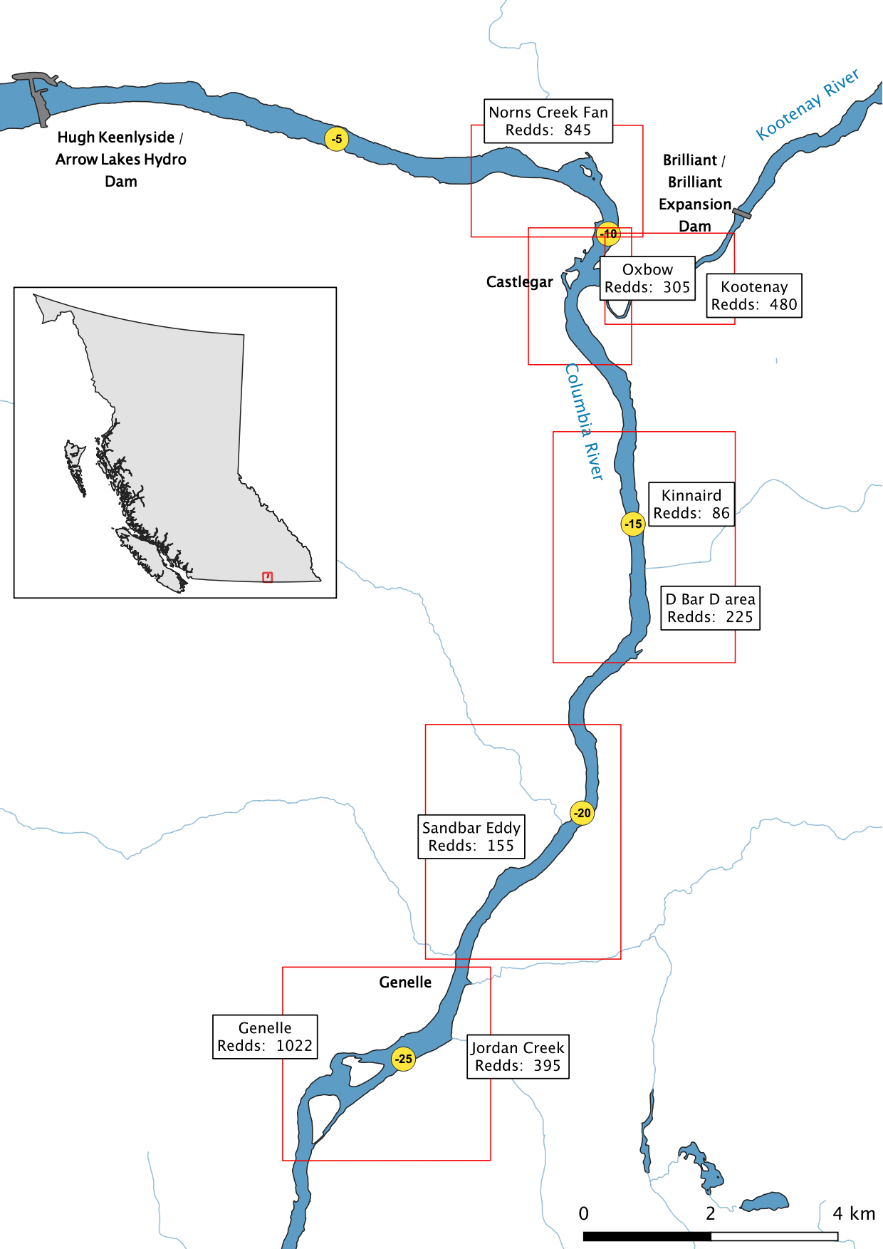
Figure 1. Overview map of the Lower Columbia River and Lower Kootenay River study area with peak count redd numbers at key areas.
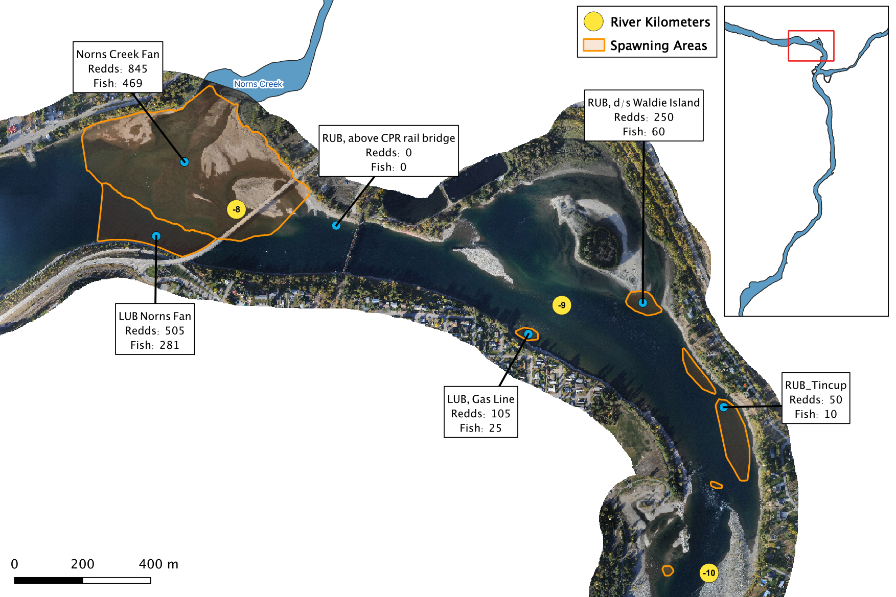
Figure 2. A map of peak fish and redd counts for the Lower Columbia River.
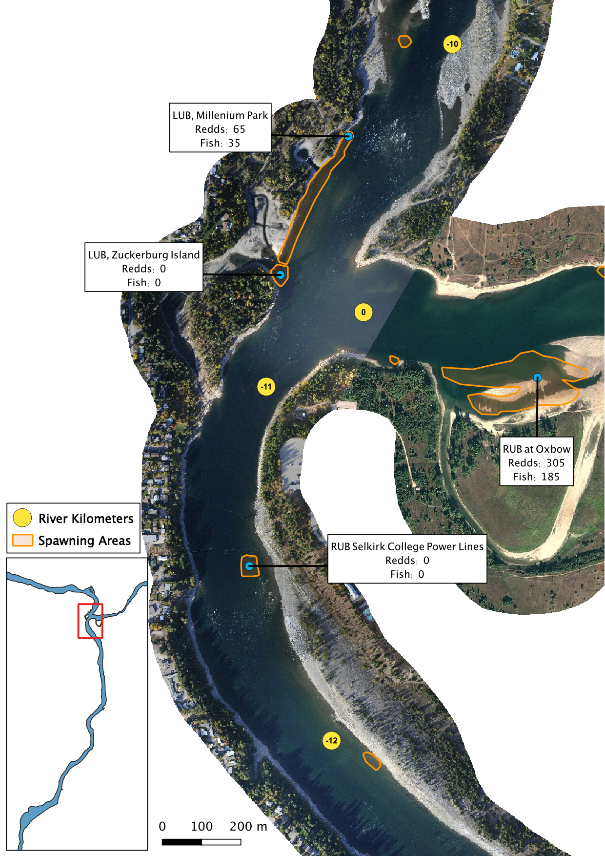
Figure 3. A map of peak fish and redd counts for the Lower Columbia River.
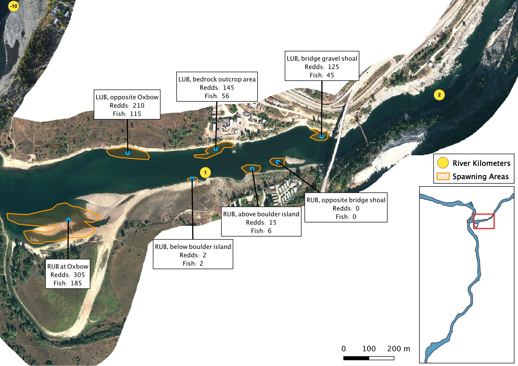
Figure 4. A map of peak fish and redd counts for the Lower Kootenay River.
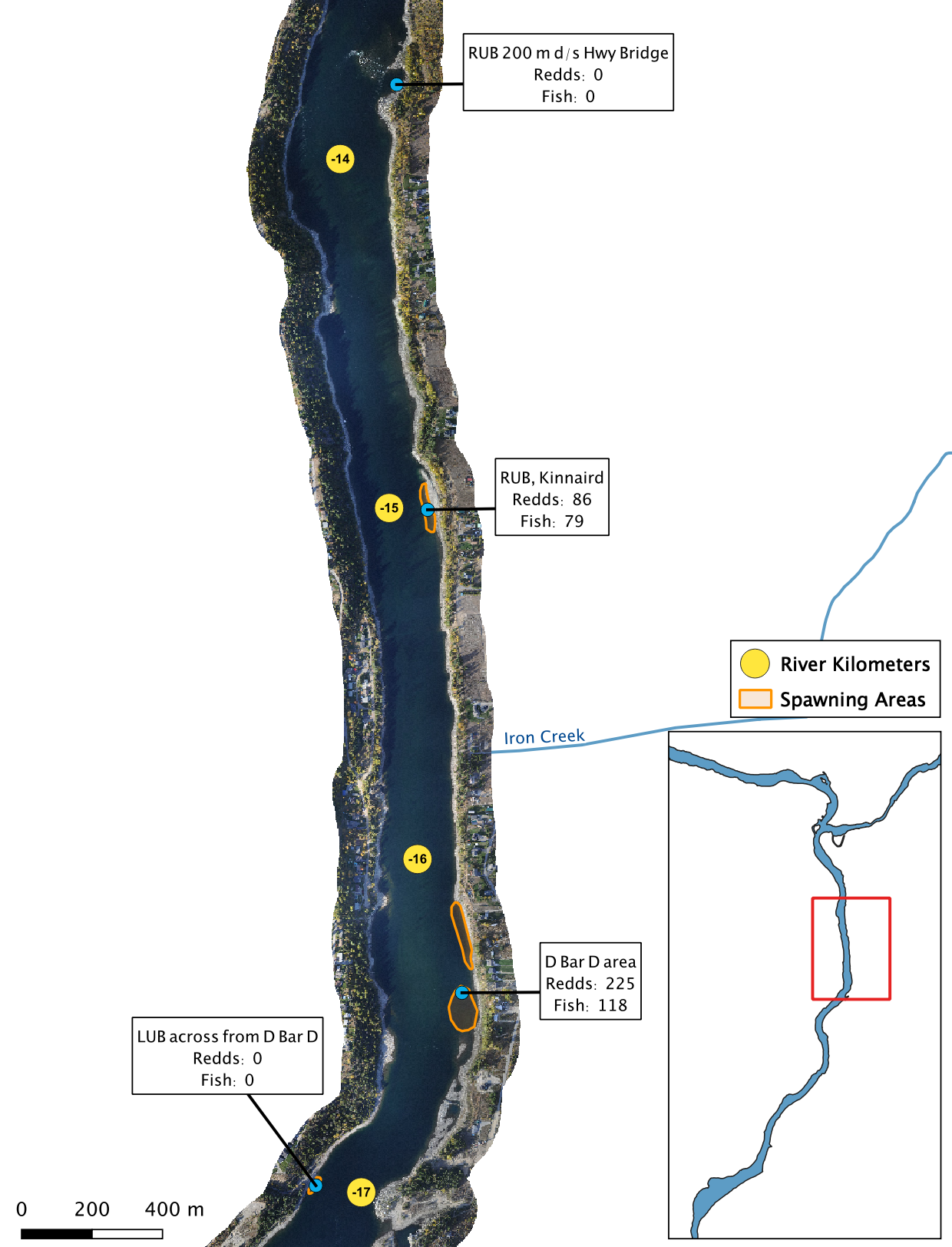
Figure 5. A map of peak fish and redd counts for the Lower Columbia River.
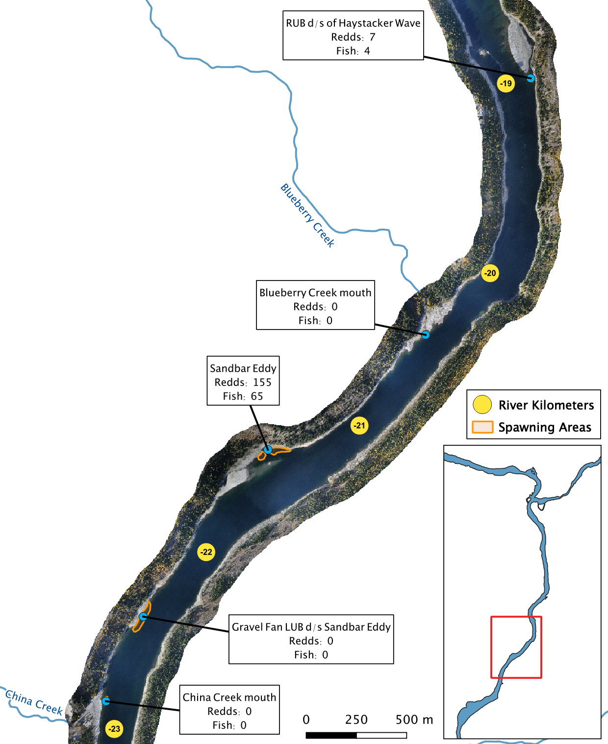
Figure 6. A map of peak fish and redd counts for the Lower Columbia River.
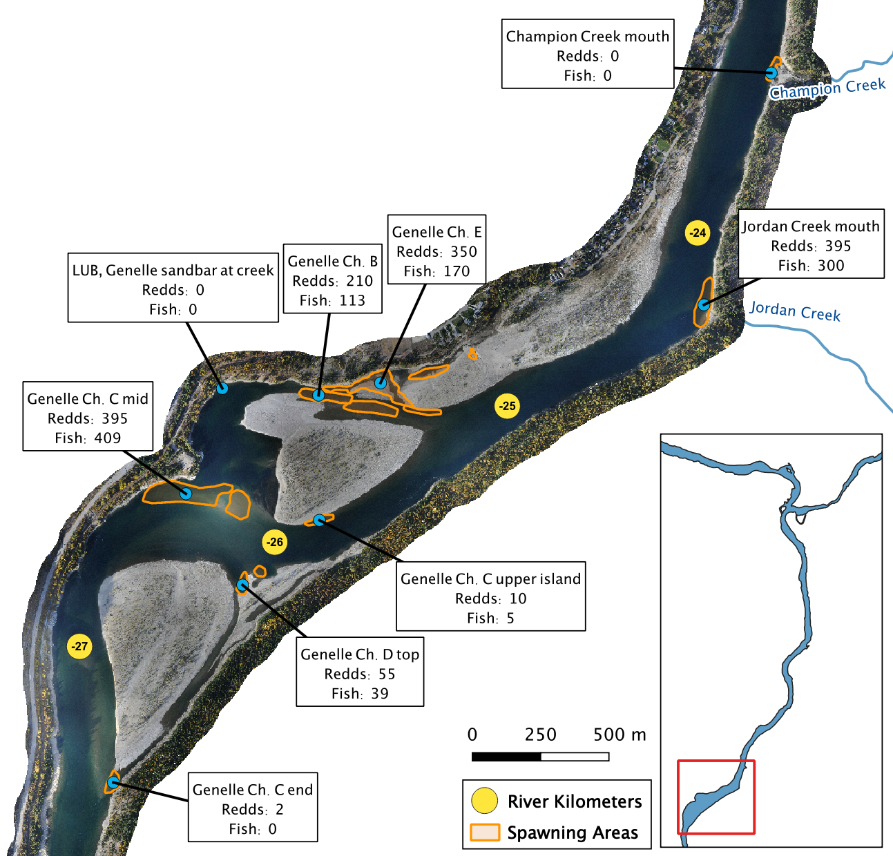
Figure 7. A map of peak fish and redd counts for the Lower Columbia River.
Stations
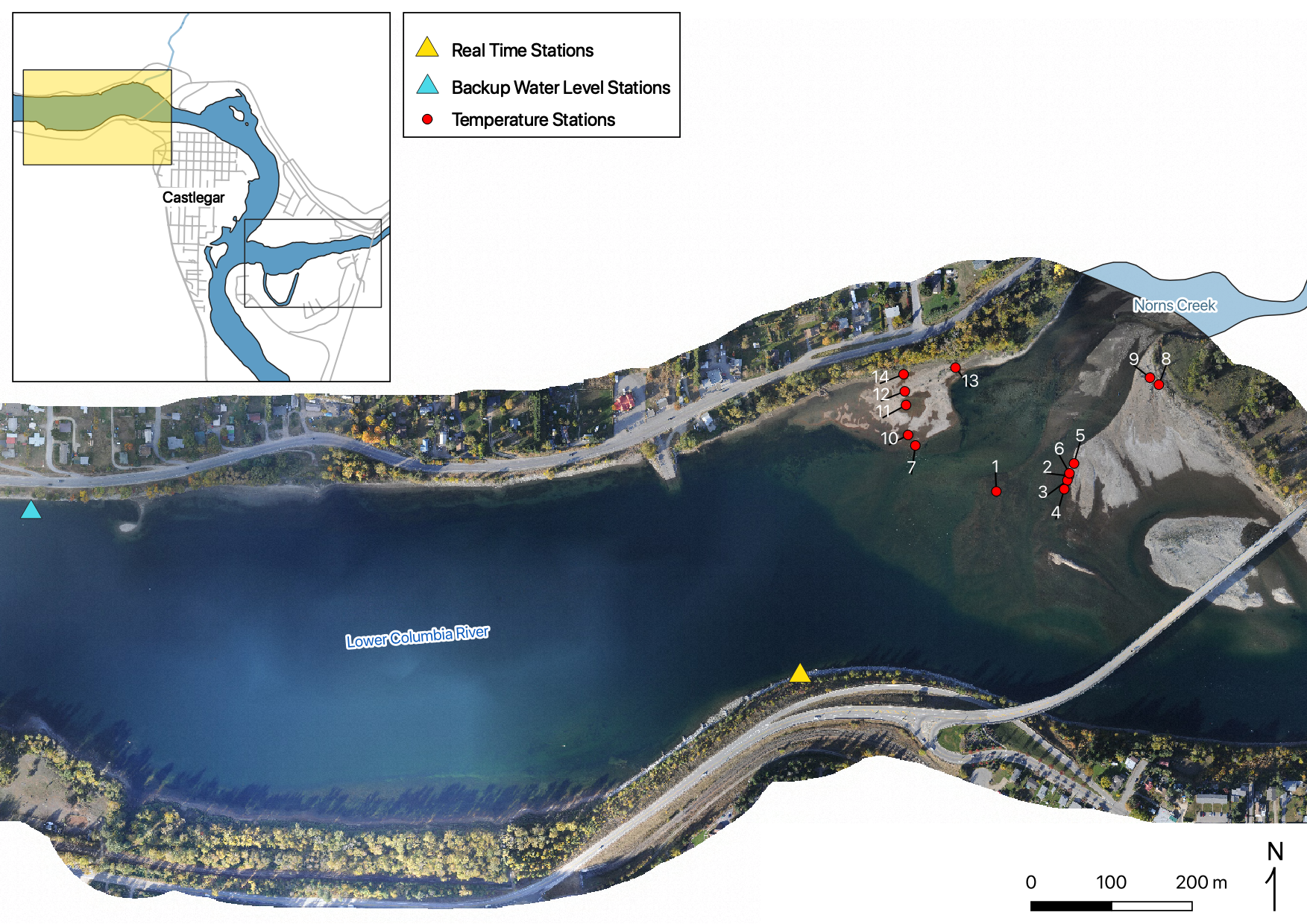
Figure 8. real time and temperature stations on the LCR at Norns Creek Fan.
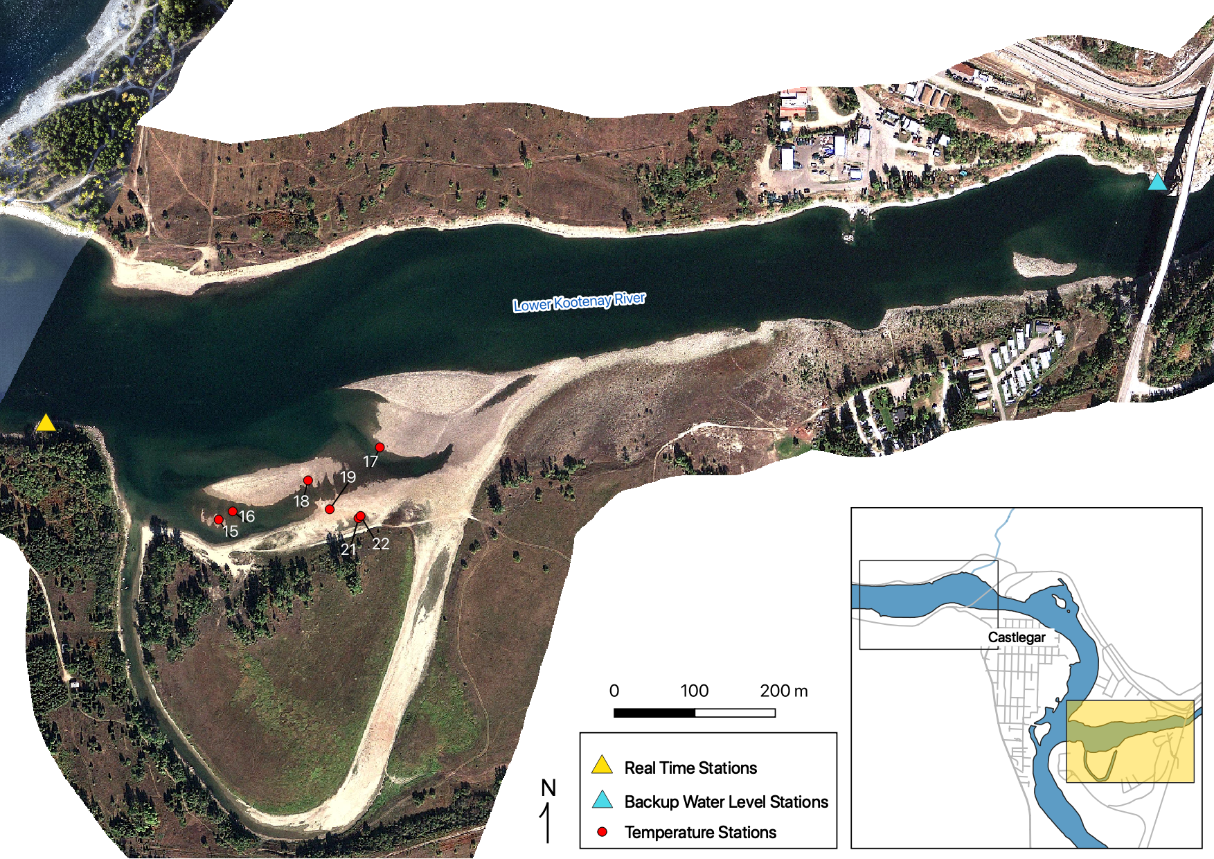
Figure 9. real time and temperature stations on the LKR at Oxbow.
Sensor Data
Real Time Stations
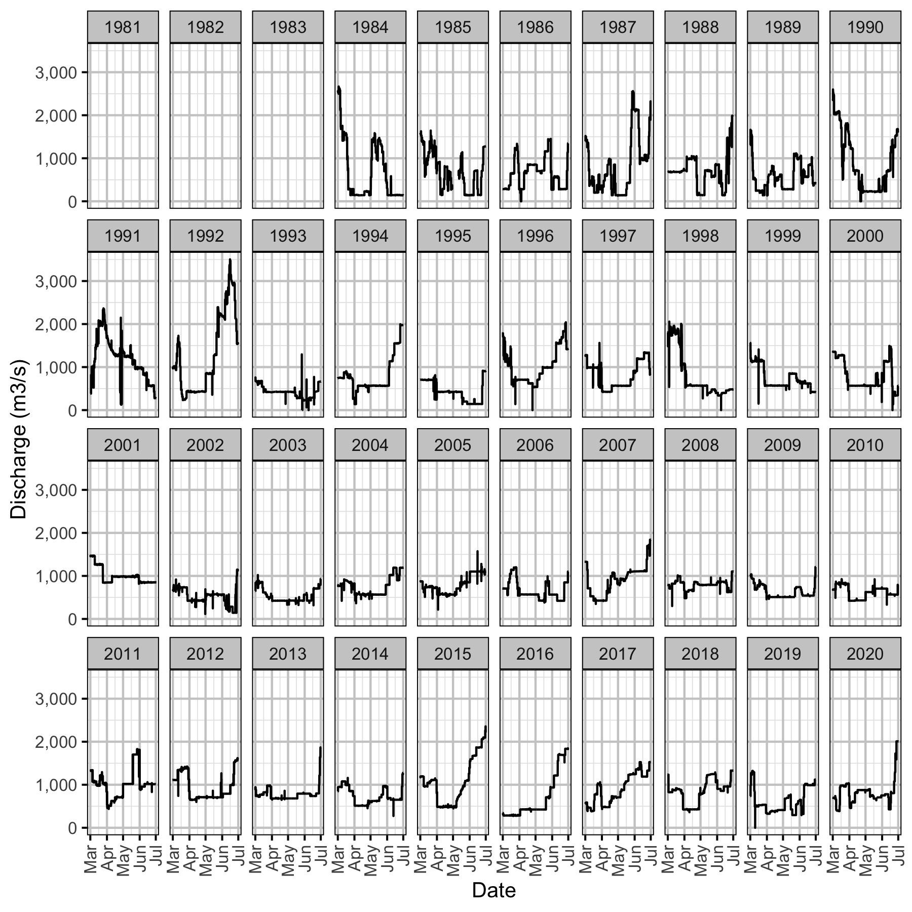
Figure 10. Hugh L. Keenleyside Dam discharge by date and year.
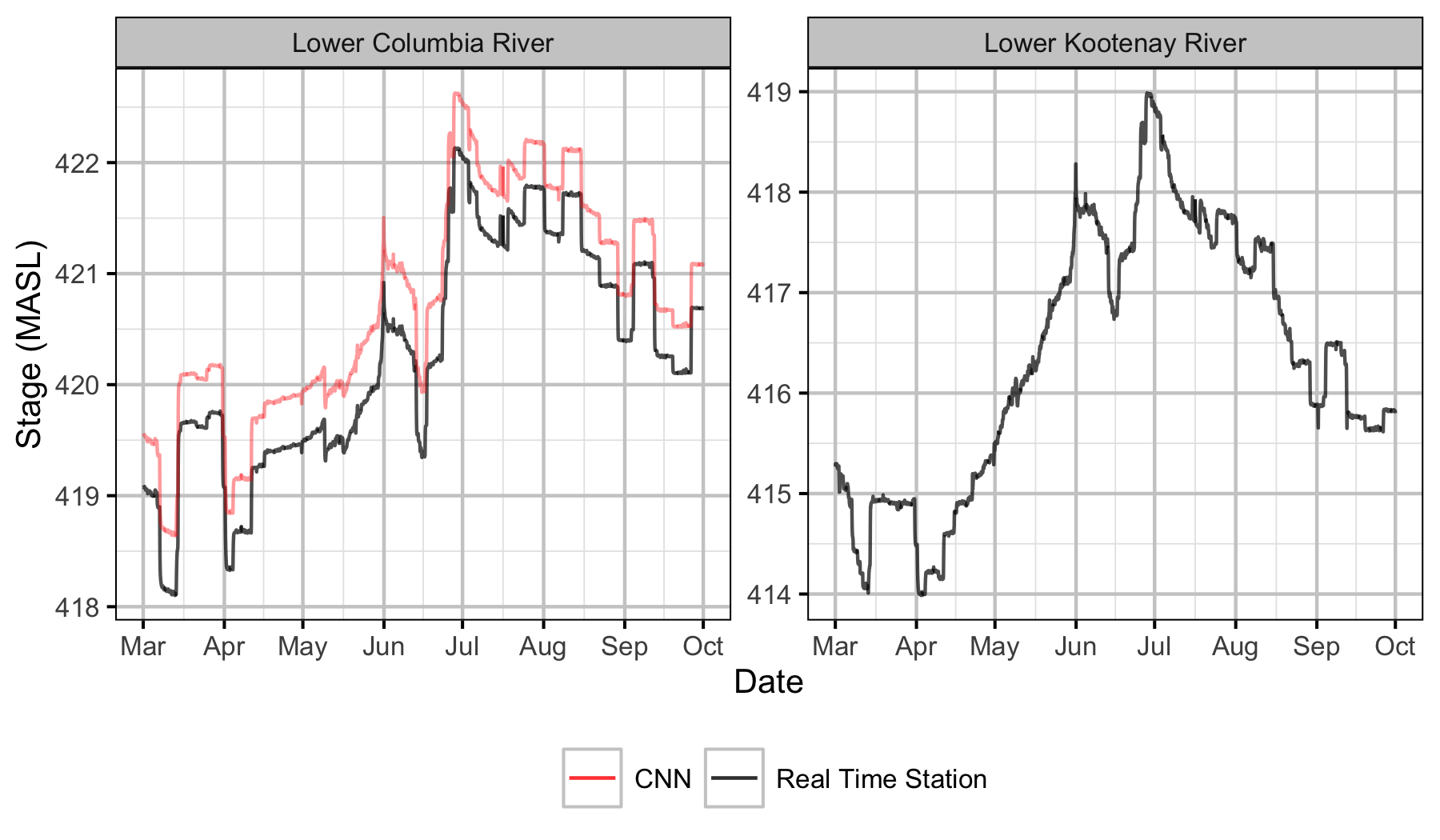
Figure 11. Water elevation by river where Lower Columbia River is Norns Creek Fan and Lower Kootenay River is the Kootenay Oxbow.
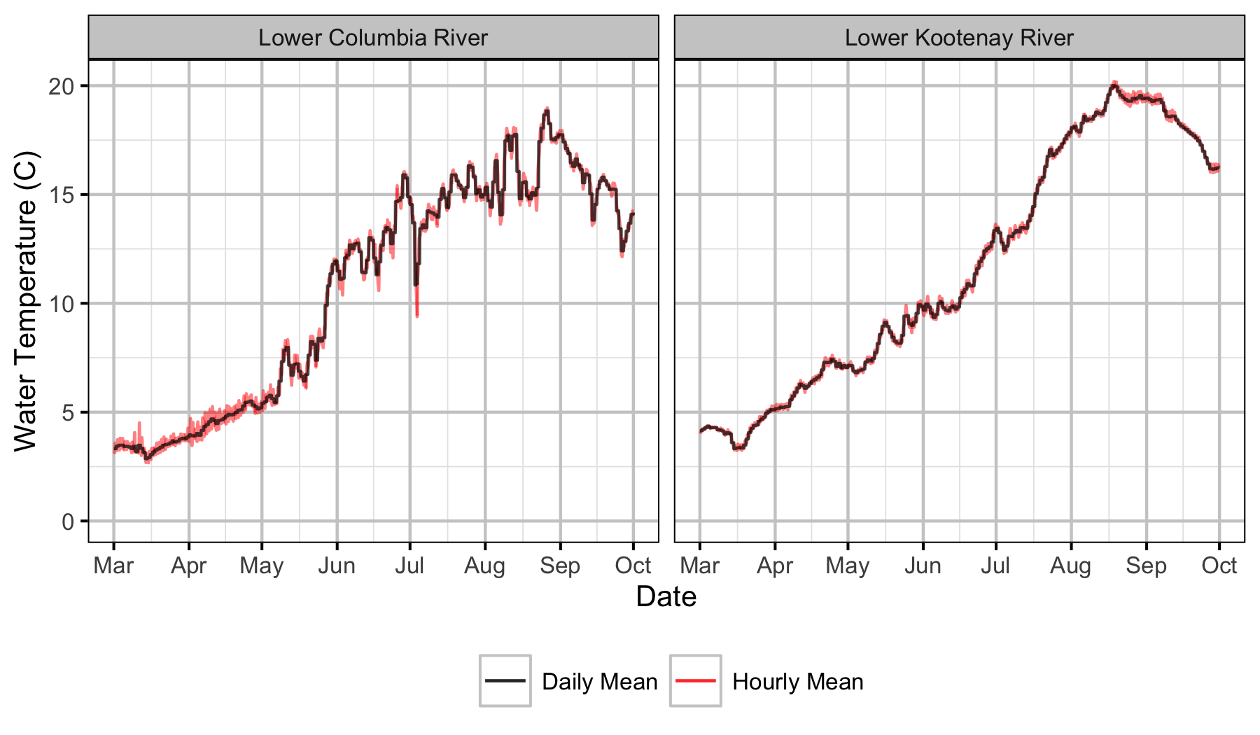
Figure 12. Water temperature by river where Lower Columbia River is Norns Creek Fan and Lower Kootenay River is the Kootenay Oxbow.
Dewatering
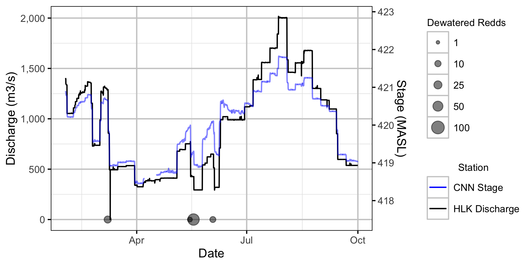
Figure 13. Major dewatering events for 2019 in relation to the LCR and LKR hydrographs.
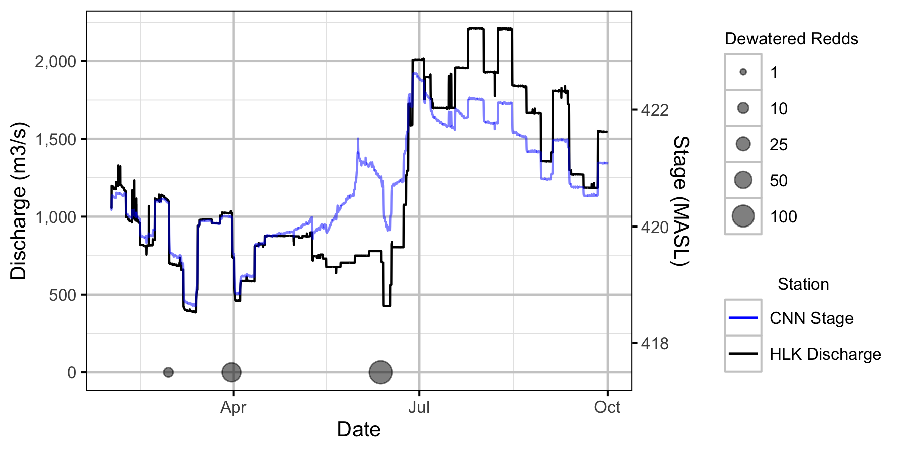
Figure 14. Major dewatering events for 2020 in relation to the LCR and LKR hydrographs.
Area-Under-The-Curve
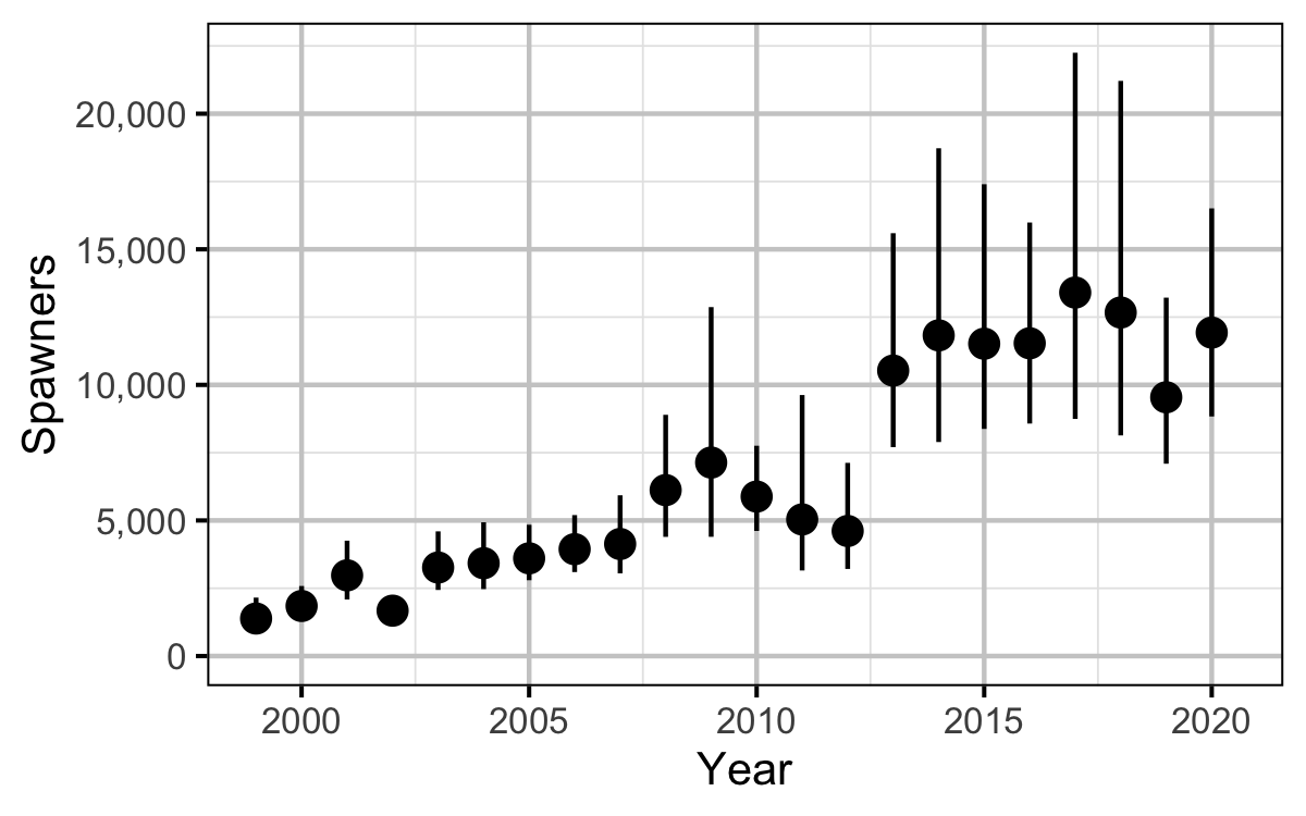
Figure 15. Estimated total spawner abundance by year (with 95% CIs).
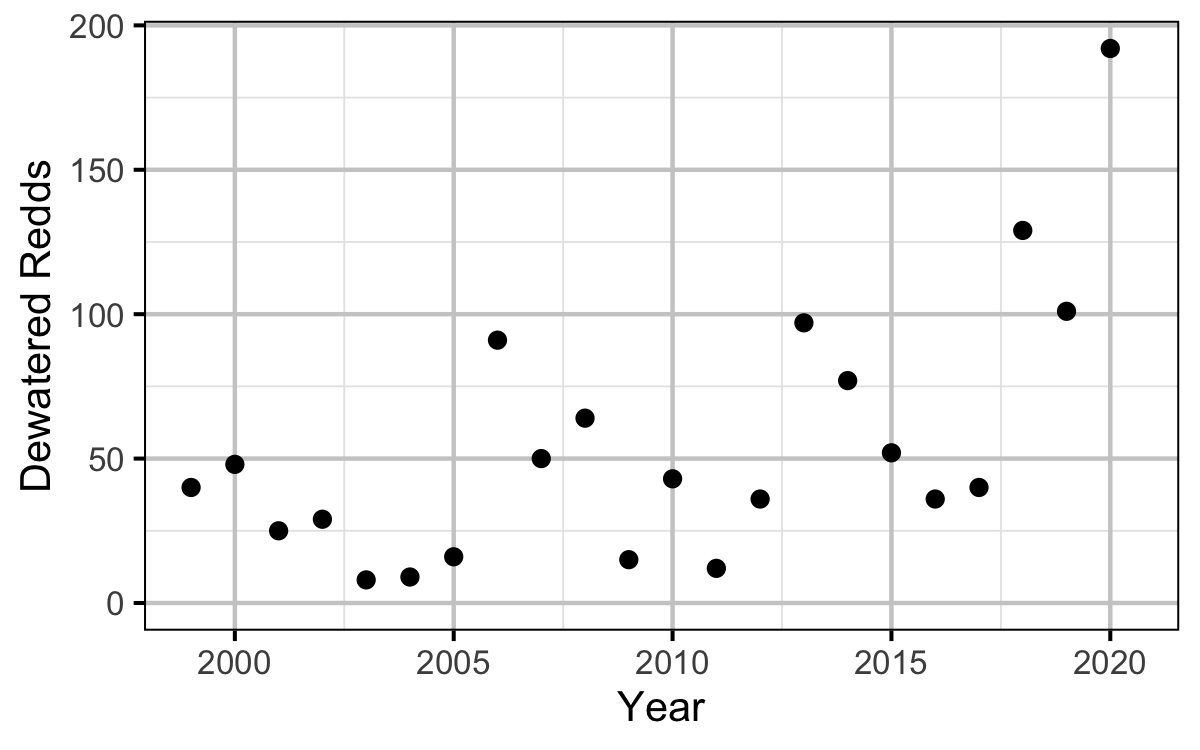
Figure 16. Dewatered redds by year.
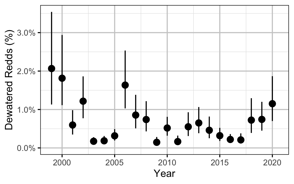
Figure 17. Estimated percent redd dewatering by year (with 95% CIs).
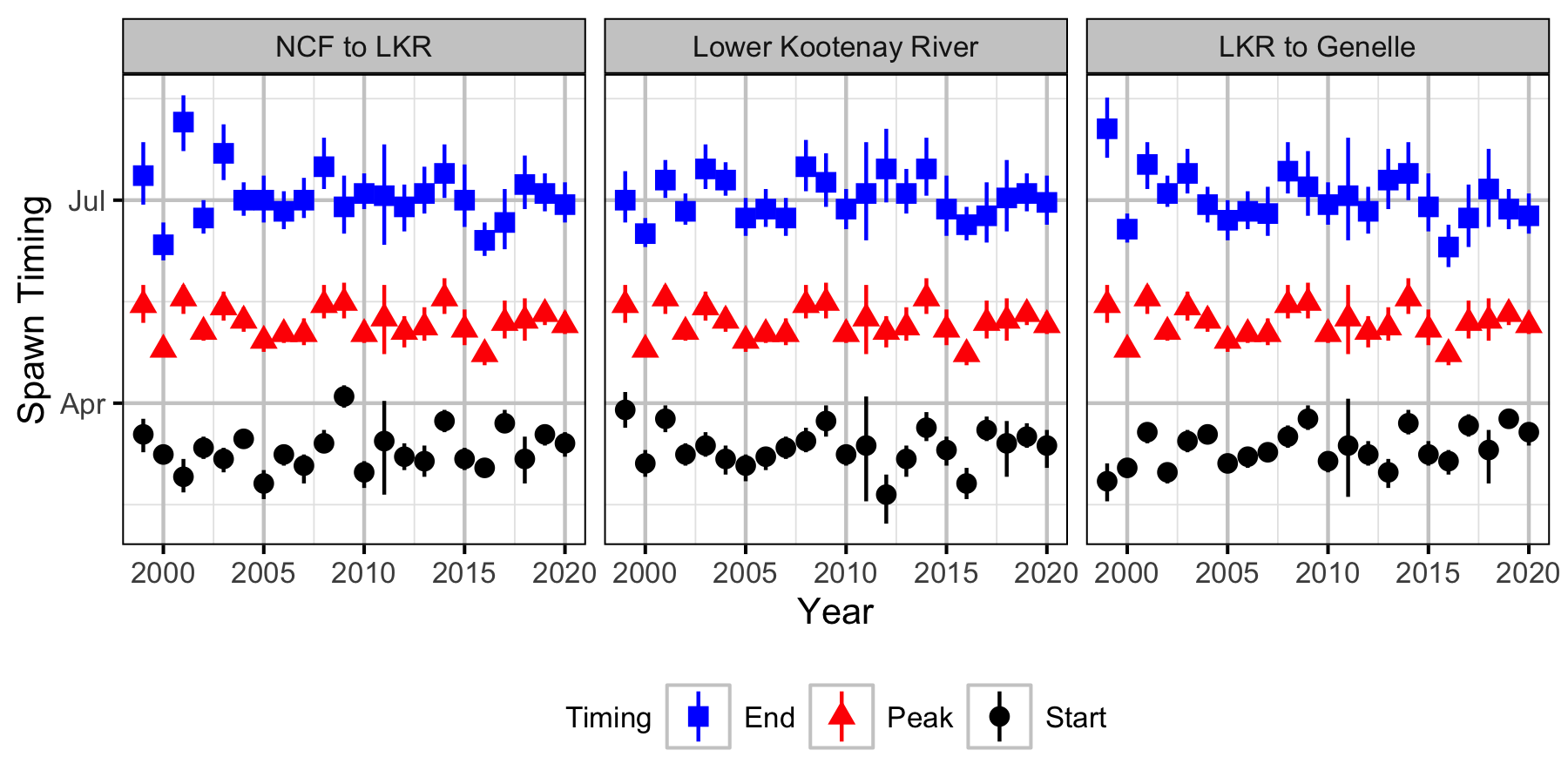
Figure 18. Estimated start (2.5% Fishs arrived), peak and end (2.5% of Fishs remaining) spawn timing by year (with 95% CIs).
Norns Creek Fan
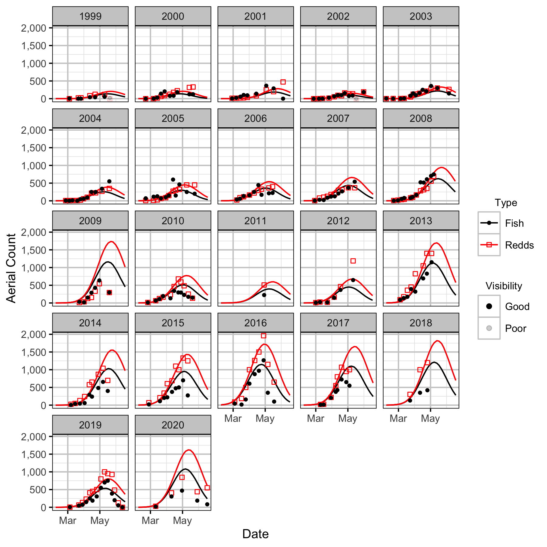
Figure 19. Predicted and actual aerial fish and redd counts at Norns Creek Fan by date and year.
NCF To LKR
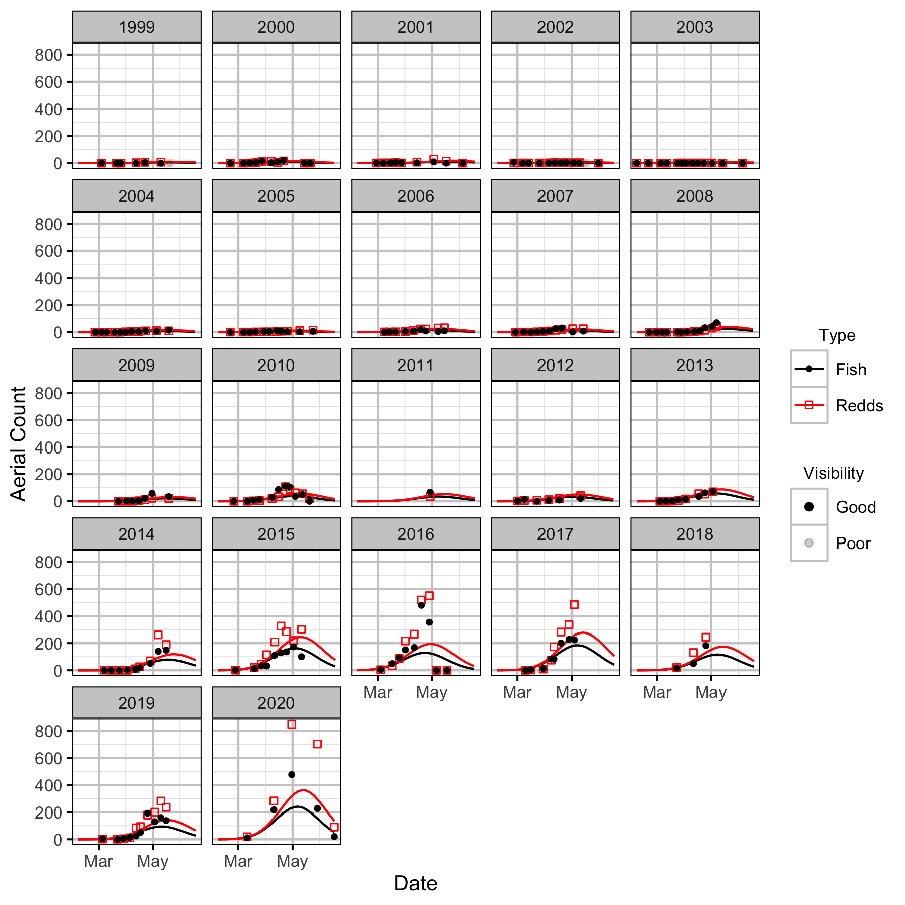
Figure 20. Predicted and actual aerial fish and redd counts at NCF to LKR by date and year.
Lower Kootenay River
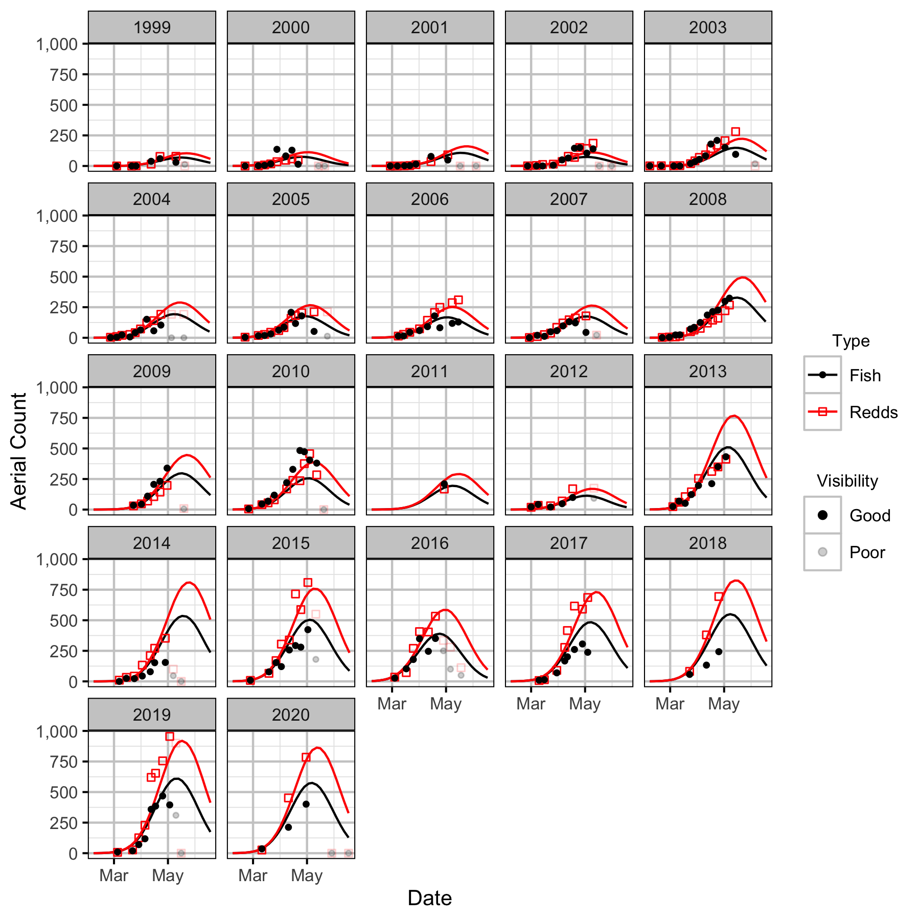
Figure 21. Predicted and actual aerial fish and redd counts at Lower Kootenay River by date and year.
LKR To Genelle
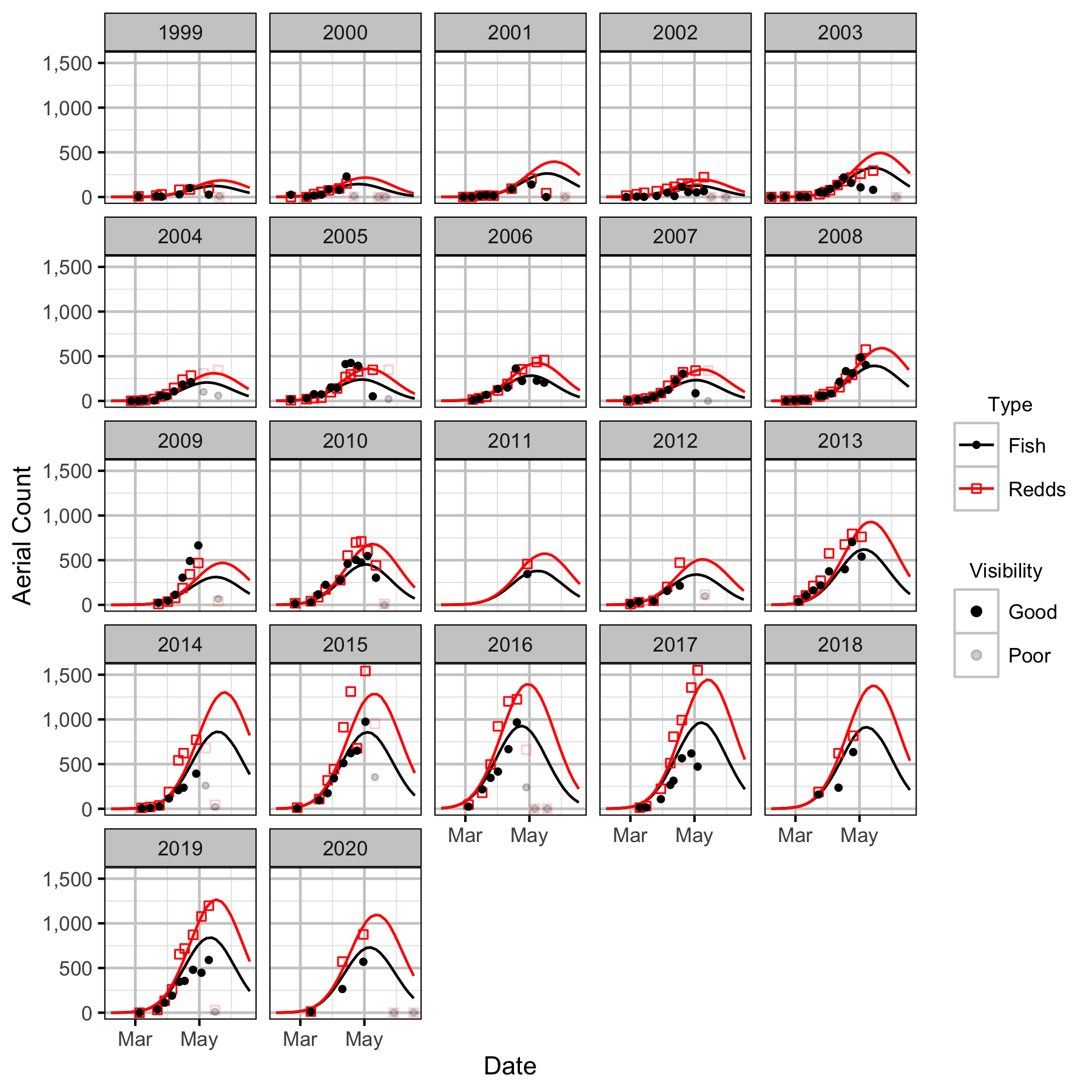
Figure 22. Predicted and actual aerial fish and redd counts at LKR to Genelle by date and year.
Genelle
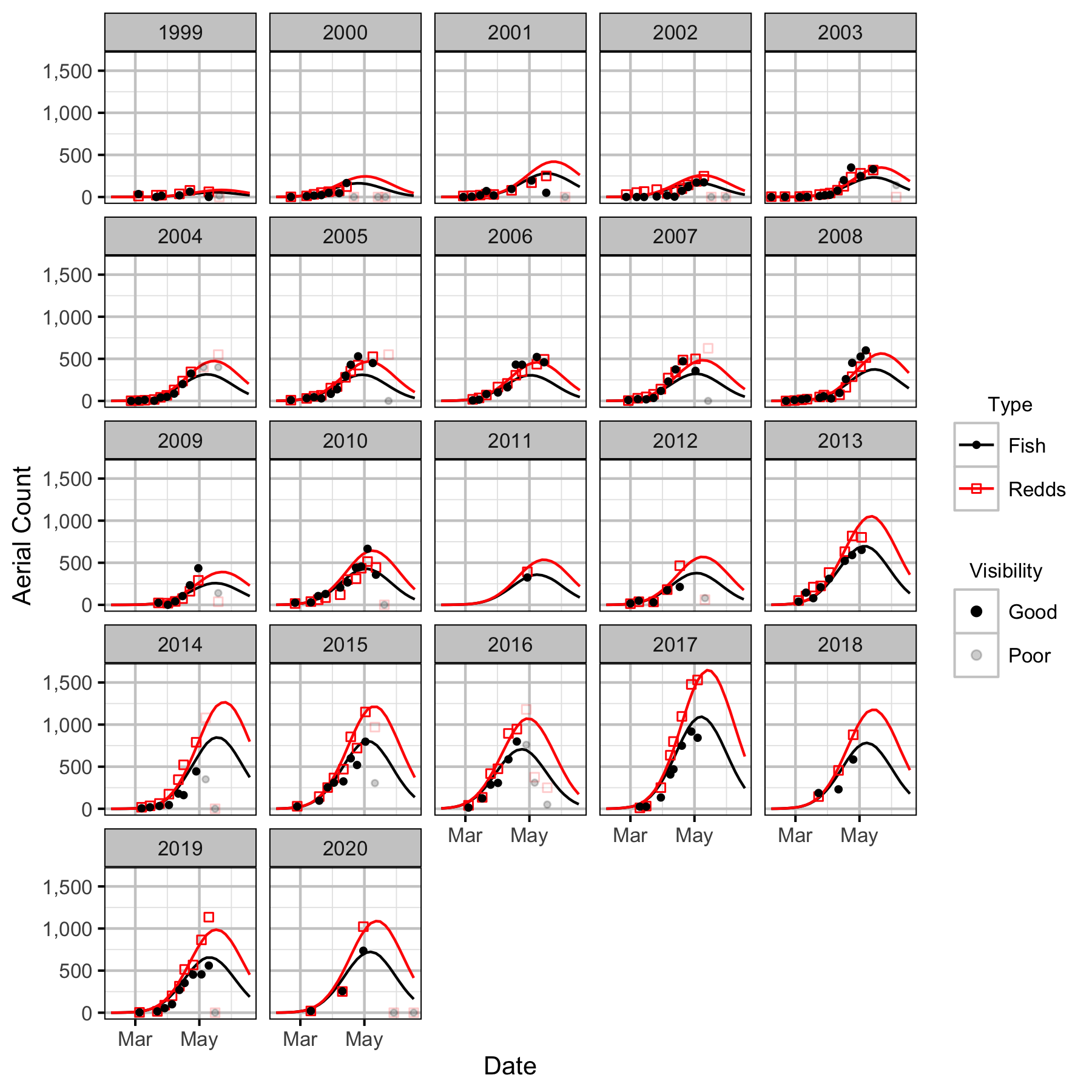
Figure 23. Predicted and actual aerial fish and redd counts at Genelle by date and year.
White Sturgeon
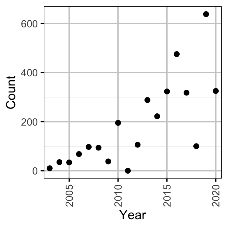
Figure 24. Peak river sturgeon counts by year.
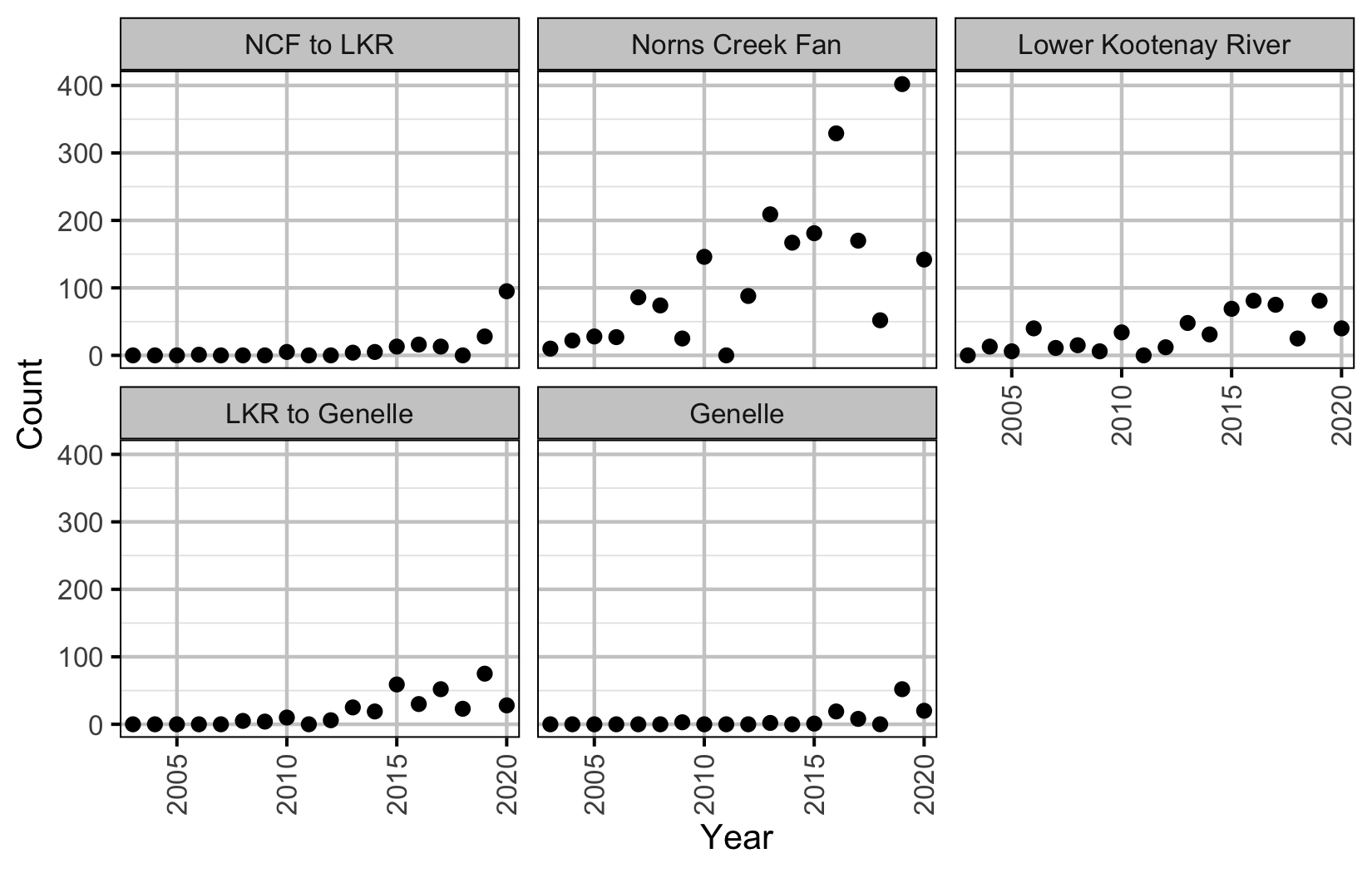
Figure 25. Peak sturgeon counts by section and year.
Drone Counts
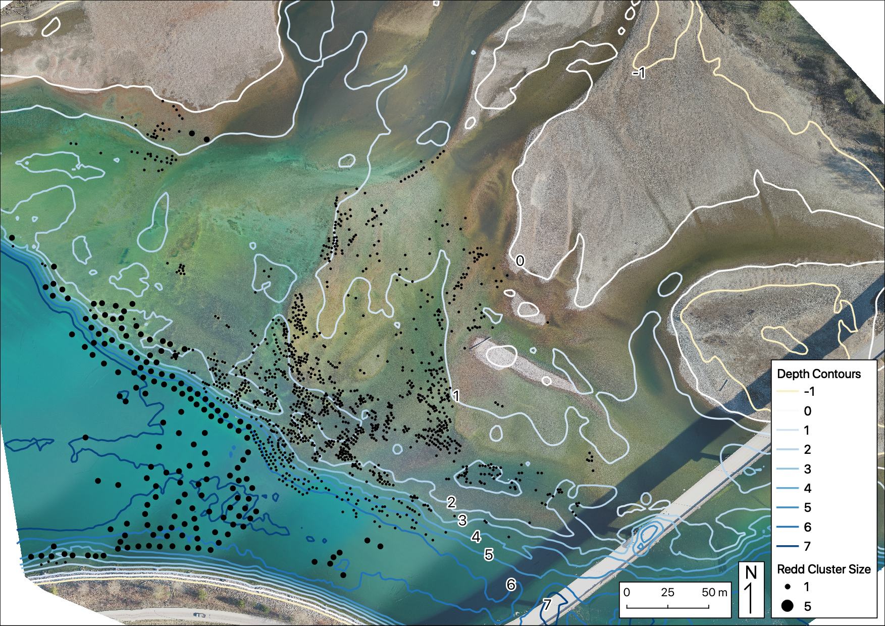
Figure 26. Cumulative redds identified over five drone surveys at Norns Creek Fan, and left upstream bank at Norns Creek Fan: April 21st, April 29th, May 12th, May 28th, and June 15th.
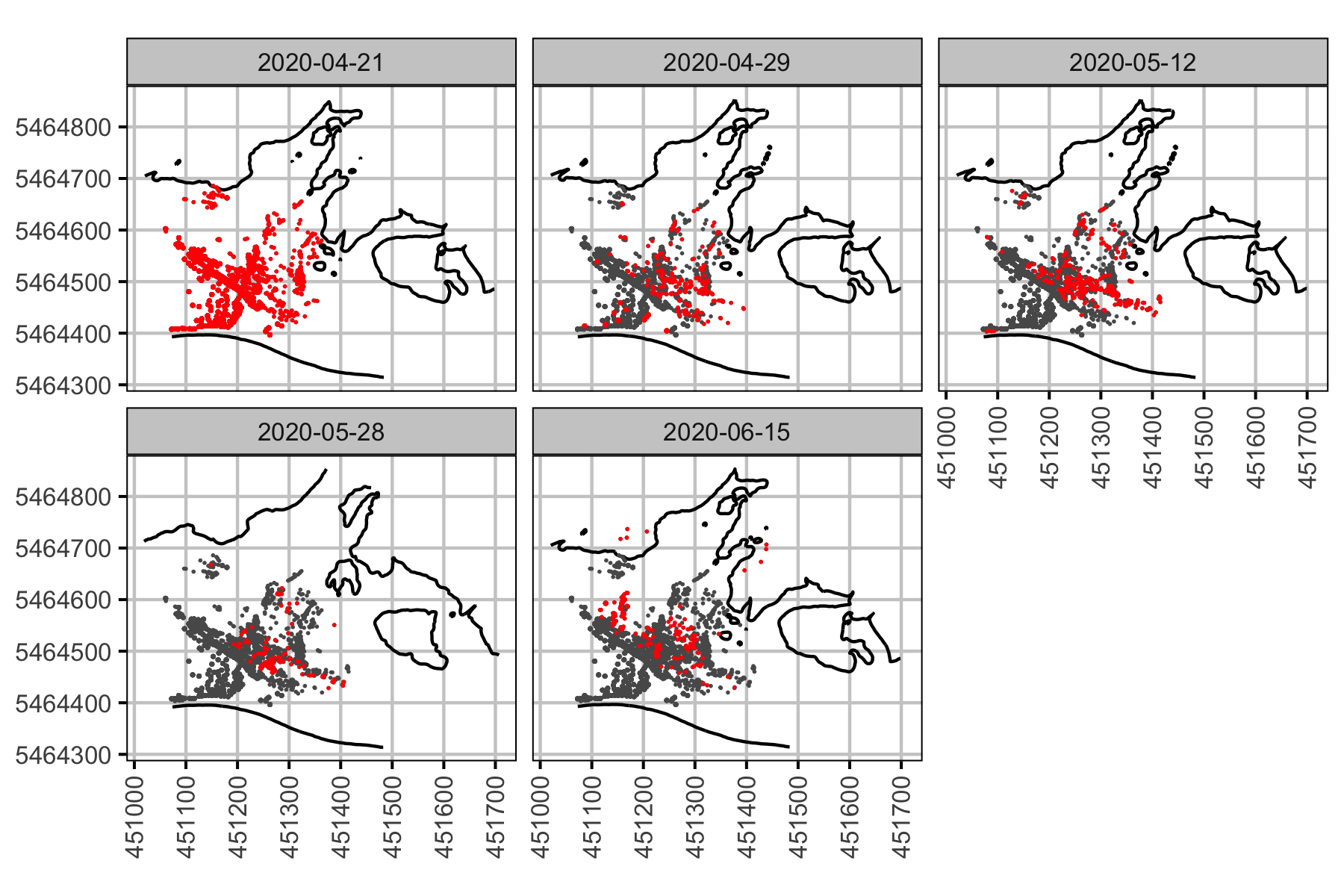
Figure 27. Accumulation of drone counted redds by date, with new redds highlighted. The wetted edge contour is shown for each survey date.
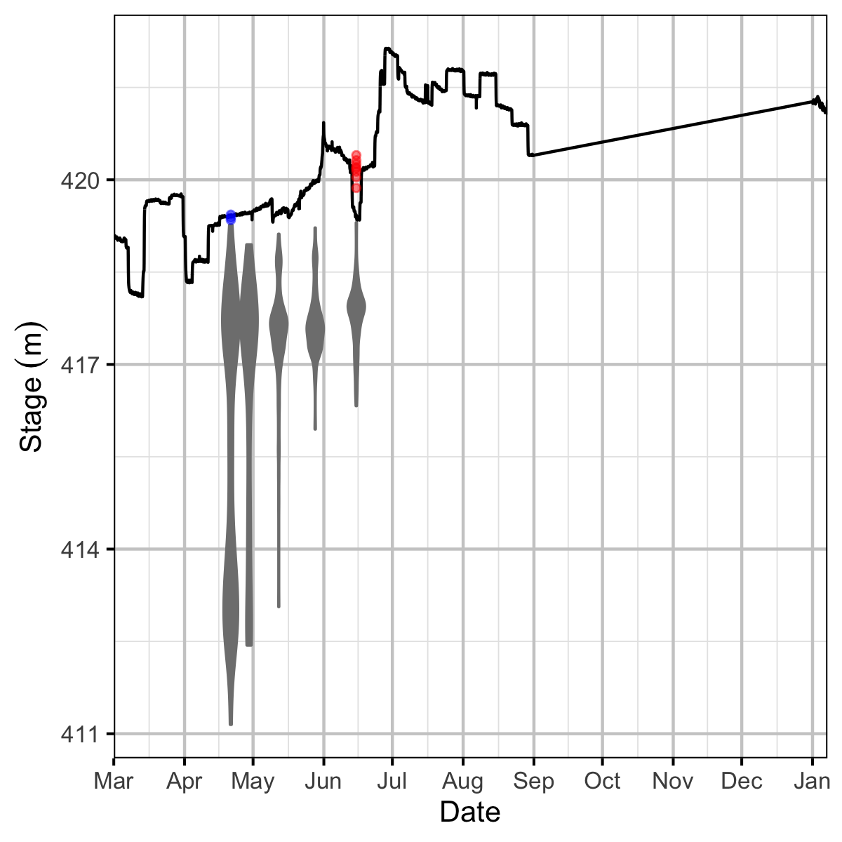
Figure 28. Elevational distribution of newly detected drone surveyed redds at Norns Creek Fan by survey date. Drone surveyed redds that were subsequently dewatered based on the stage elevation are blue. Redds that were identified during the ground surveys are colored red.
Stock-Recruitment
Spawners
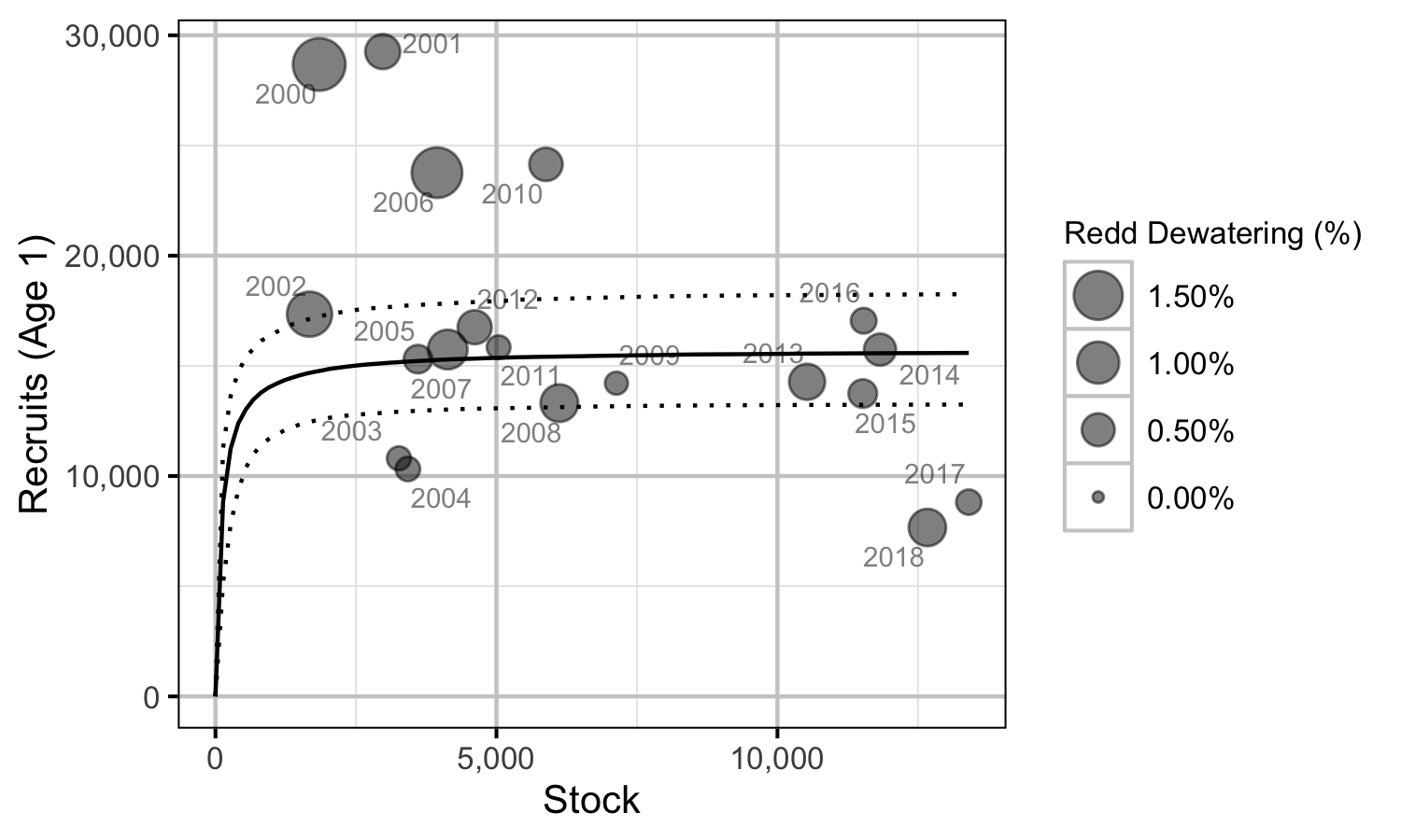
Figure 29. Predicted stock-recruitment relationship from spawners to subsequent age-1 recruits by spawn year (with 95% CIs).
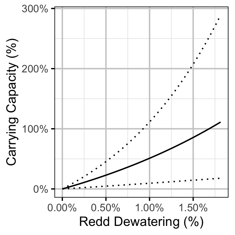
Figure 30. Predicted age-1 recruits carrying capacity by percentage egg dewatering (with 95% CRIs).
Eggs
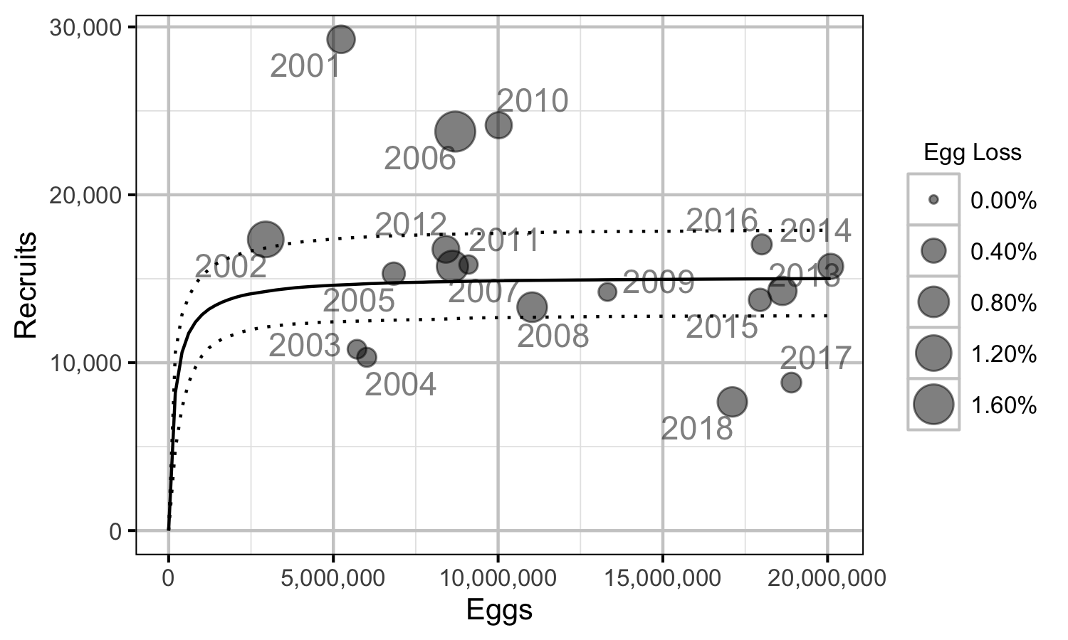
Figure 31. Predicted stock-recruitment relationship by spawn year (with 95% CRIs).
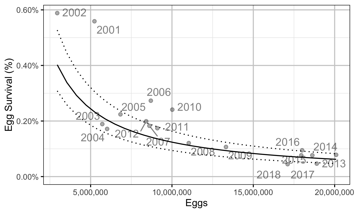
Figure 32. Predicted egg to age-1 survival by total egg deposition (with 95% CRIs).
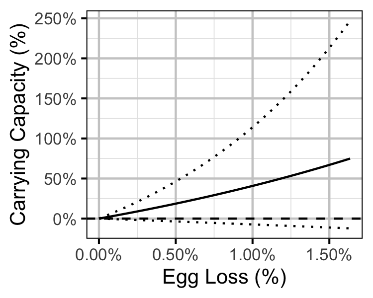
Figure 33. Predicted effect of egg loss on the age-1 carrying capacity (with 95% CRIs).
Egg Mortality
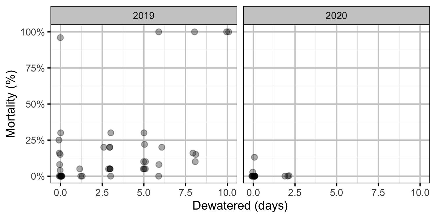
Figure 34. Observed egg mortality excavated redds by days dewatered.
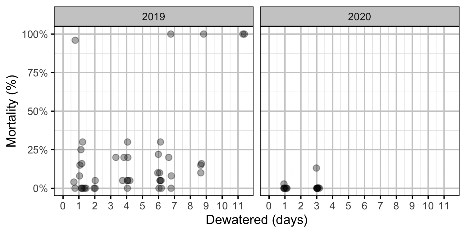
Figure 35. Observed egg mortality excavated redds by days dewatered.
Stage
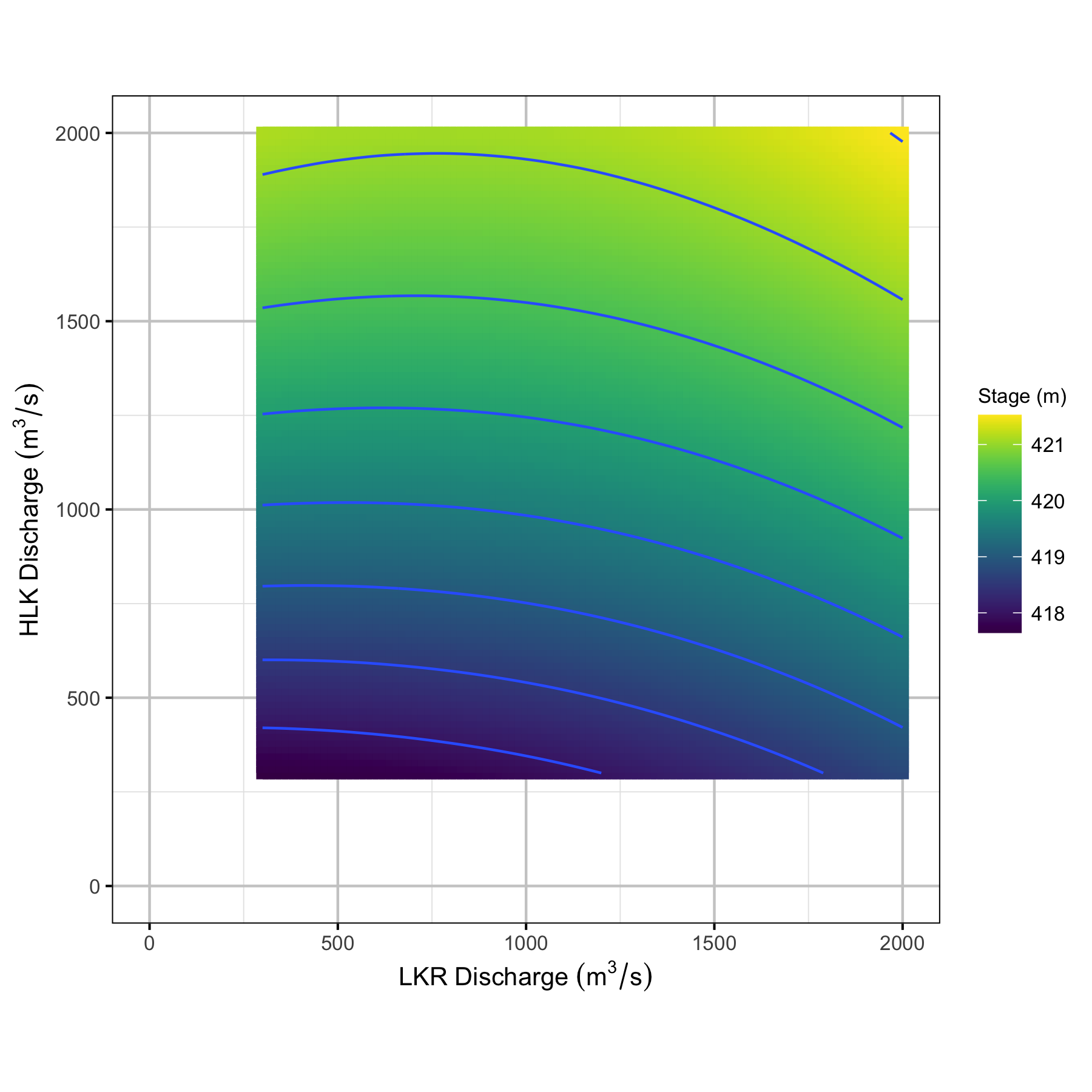
Figure 36. Predicted stage height at CNN by discharge from LKR and HLK Dam.
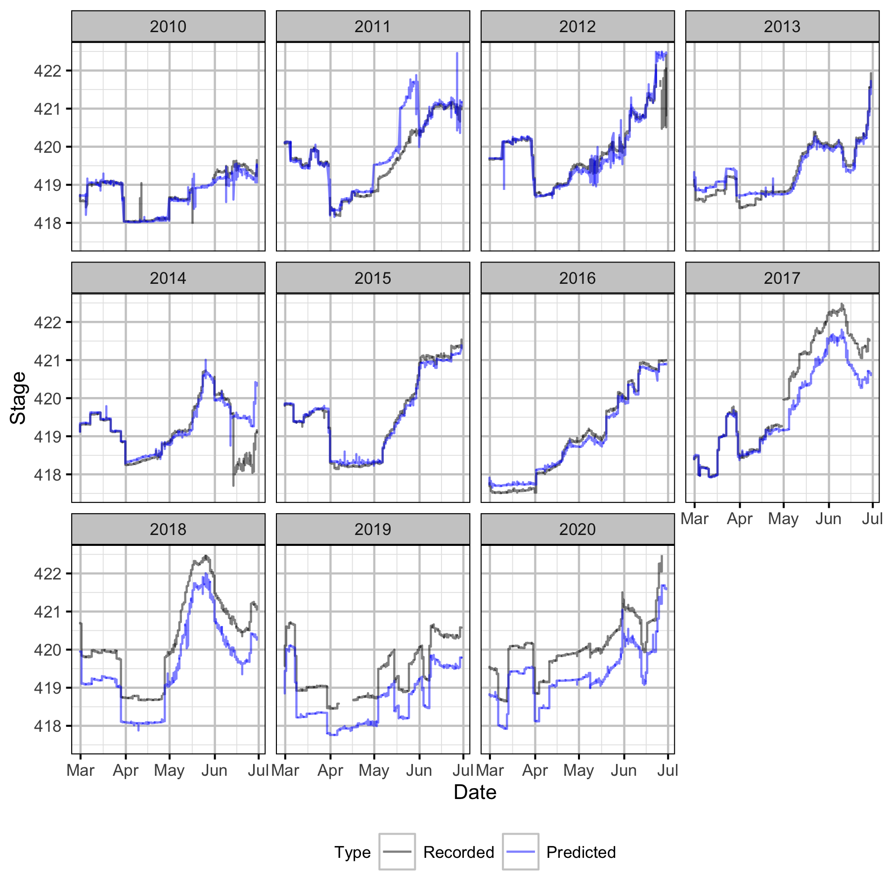
Figure 37. Recorded and uncorrected predicted hourly stage height at CNN by year.
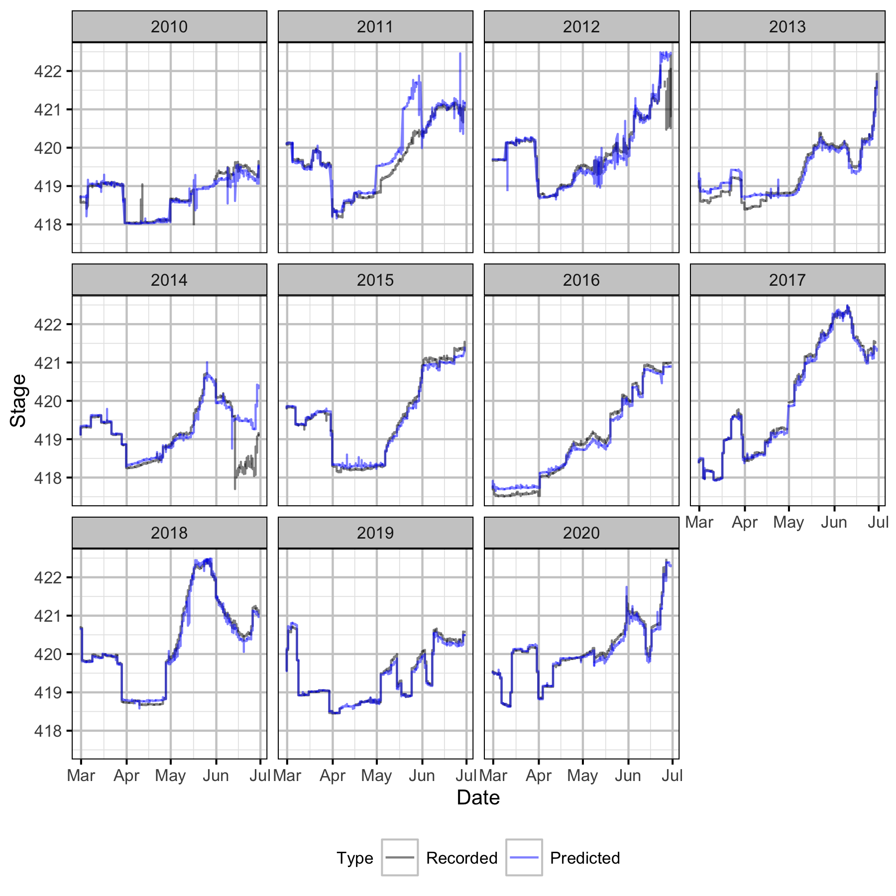
Figure 38. Recorded and predicted hourly stage height at CNN by year.
Acknowledgements
The organisations and individuals whose contributions have made this analysis report possible include:
- BC Hydro
- Philip Bradshaw
- James Baxter
- Guy Martel
- Margo Dennis
- Darin Nishi
- Nuupqu
- Mark Fjeld
- Natalie Morrison
- Mountain Water Research
- Jeremy Baxter
- Poisson Consulting
- Robyn Irvine
- Dam Helicopters
- Duncan Wassick
- Highland Helicopters
- Phil Hocking
- Mark Homis
- Golder Associates
- Dustin Ford
- Demitria Burgoon
- David Roscoe
- Additional Support
- Clint Tarala
- Crystal Lawrence
- Gary Pavan
- Gerry Nellestijn
- Jay Bowers