Lower Columbia River Sculpin and Dace Stranding Analysis 2013
The suggested citation for this analytic report is:
Thorley, J.L. (2014) Lower Columbia River Sculpin and Dace Stranding Analysis 2013. A Poisson Consulting Analysis Report. URL: https://www.poissonconsulting.ca/f/1090742912.
Background
Discharge reductions associated with the operation of HLK and Brilliant Dams on the Lower Columbia River, British Columbia, can cause fish stranding.
The management question the current analysis attempts to answer is:
Which operations, and at what season, pose the highest risk of stranding or interference with the normal life cycles of sculpins and dace?
Methods
Data Collection
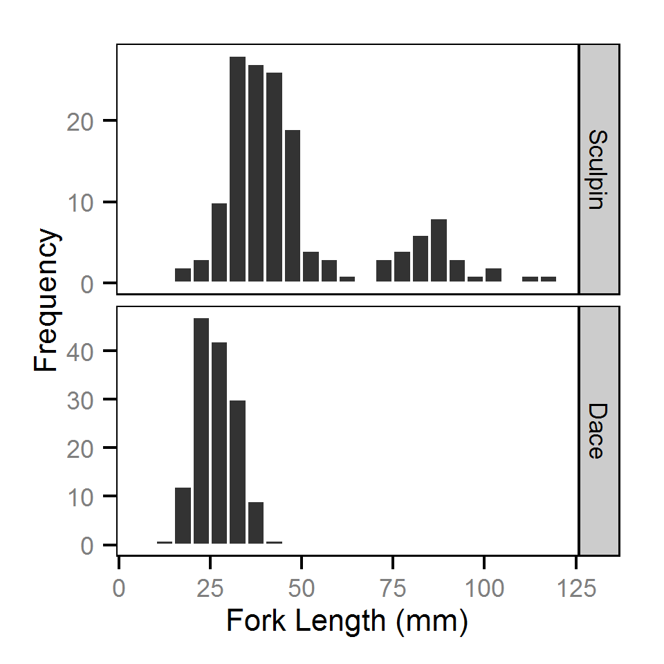
Following reduction events, crews are dispatched to salvage stranded fish from areas of concern. At each site the crew record the number of pools, the number of pools surveyed and the number of fish counted by species, genus, family or all species in the surveyed pools. Since 2011, the crew have also lengthed a subsample of individuals.
Data Preparation
The fish stranding data were provided by Golder Associates in the form of an Access database. The discharge data were queried from a BC Hydro database maintained by Poisson Consulting.
The data were prepared for analysis using R version 3.1.0 (Team, 2013).
Pool Stranding
During the pool stranding data preparation it was assumed that:
- Fish species code LND refers to long nose dace (LNC).
- The proportion of unidentified fish that were dace was the same as the proportion of identified fish (2.1%).
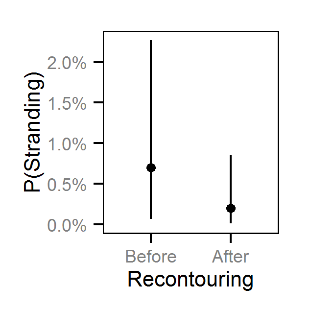
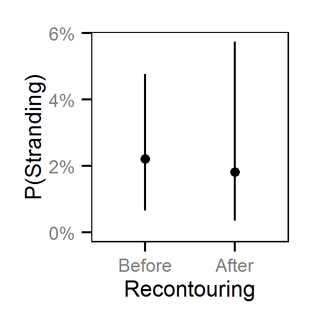
- The Genelle (Mainland) (LUB) site was recontoured in February 2003.
Discharge
During the discharge data preparation it was assumed that:
- The magnitude of a reduction event was the difference between the peak discharge in the previous 24 hours and the discharge at the time of the survey.
- The rate of a reduction event was the weighted mean hourly drop between the peak and the time of survey. Drops that were subsequently inundated prior to the survey were assigned zero weight while partially inundated drops were discounted accordingly.
- The time of a reduction event was the mean time between the peak and the survey weighted by the discounted drops.
- The delay was the number of hours between the time of the reduction event and the time of the survey.
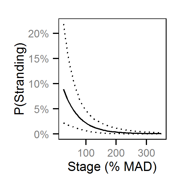
- The stage was the discharge at the time of the reduction as the percent mean annual discharge (% MAD) of the section of river to take into account differences in river size.
- The diel period was whether or not the time of reduction occurred in daylight.
Statistical Analysis
Hierarchical Bayesian models were fitted to the stranding data using R version 3.1.0 (Team, 2013) and JAGS 3.4.0 (Plummer, 2012) which interfaced with each other via jaggernaut 1.8.1 (Thorley, 2014). For additional information on hierarchical Bayesian modelling in the BUGS language, of which JAGS uses a dialect, the reader is referred to Kery and Schaub (2011) pages 41-44.
Unless specified, the models assumed vague (low information) prior distributions (Kéry and Schaub, 2011, p. 36). The posterior distributions were estimated from a minimum of 1,000 Markov Chain Monte Carlo (MCMC) samples thinned from the second halves of three chains (Kéry and Schaub, 2011, pp. 38-40). Model convergence was confirmed by ensuring that Rhat (Kéry and Schaub, 2011, p. 40) was less than 1.1 for each of the parameters in the model (Kéry and Schaub, 2011, p. 61). Model adequacy was confirmed by examination of residual plots.
The posterior distributions of the fixed (Kéry and Schaub, 2011, p. 75) parameters are summarised in terms of a point estimate (mean), lower and upper 95% credible limits (2.5th and 97.5th percentiles), the standard deviation (SD), percent relative error (half the 95% credible interval as a percent of the point estimate) and significance (Kéry and Schaub, 2011, p. 37,42).
Variable selection was achieved by dropping uninformative explanatory variables where a variable was considered to be uninformative if its percent relative error was \(\geq\) 100%. In the case of fixed effects this is approximately equivalent to dropping insignificant variables, i.e., those with a significance \(\geq\) 0.05.
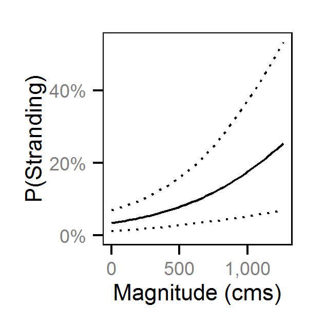
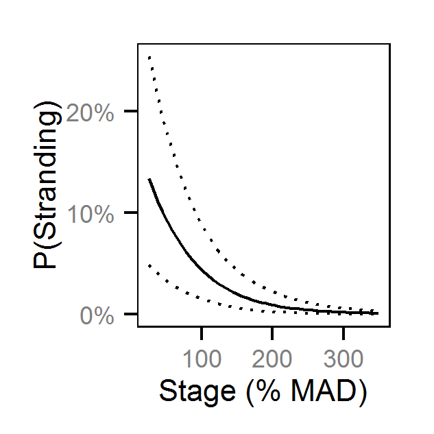
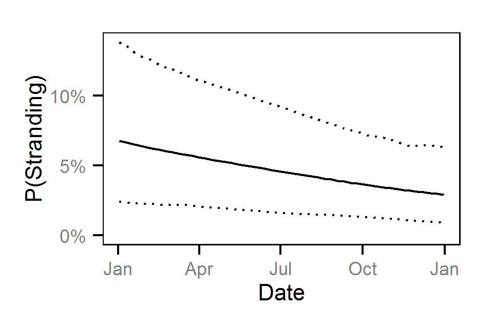
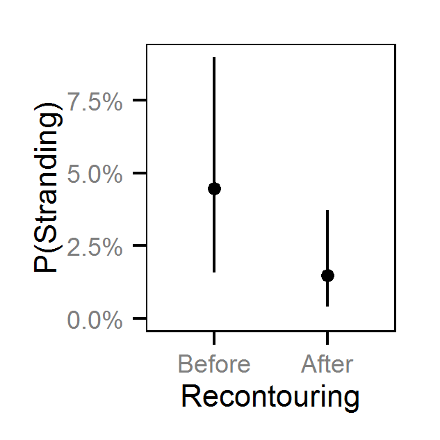
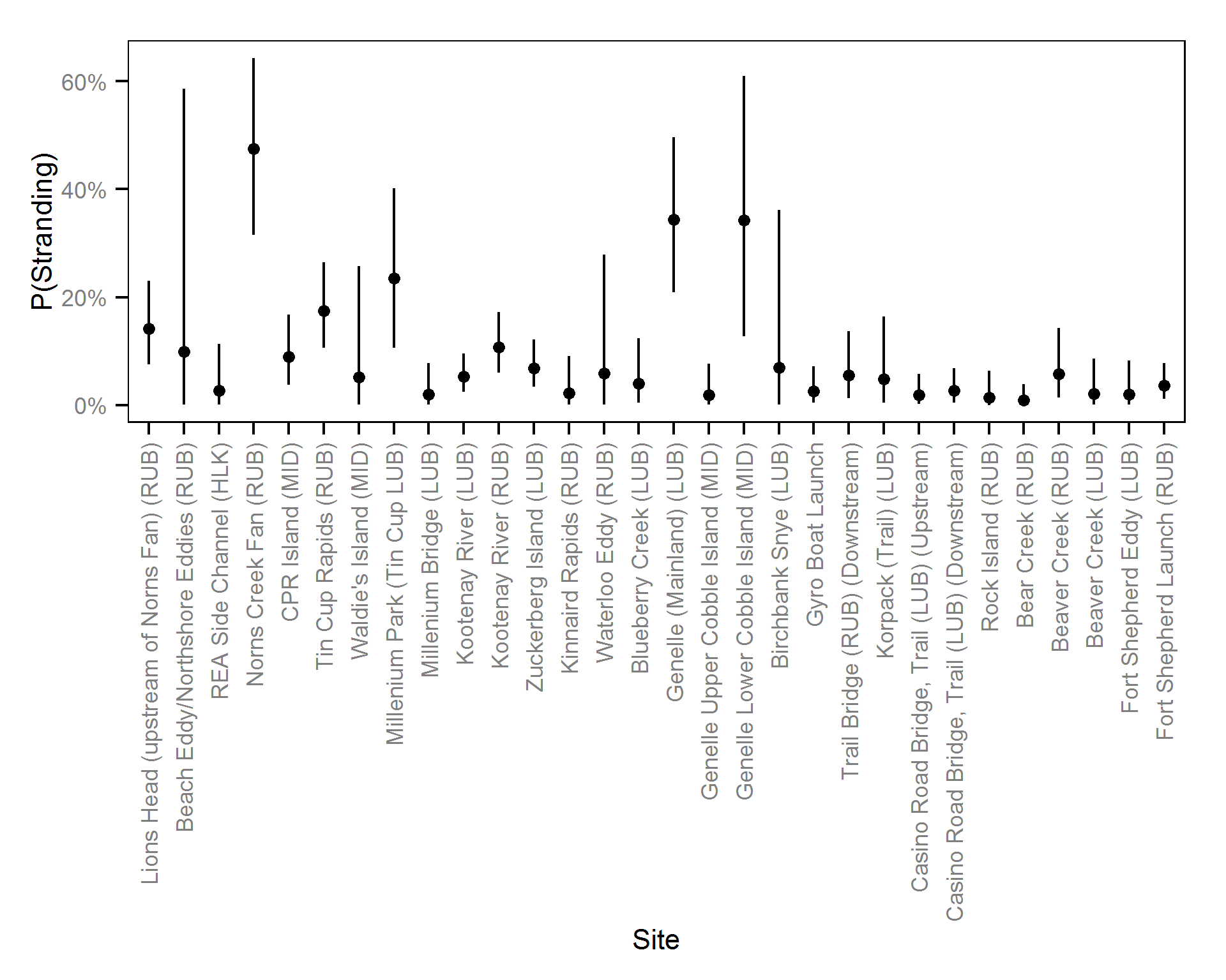
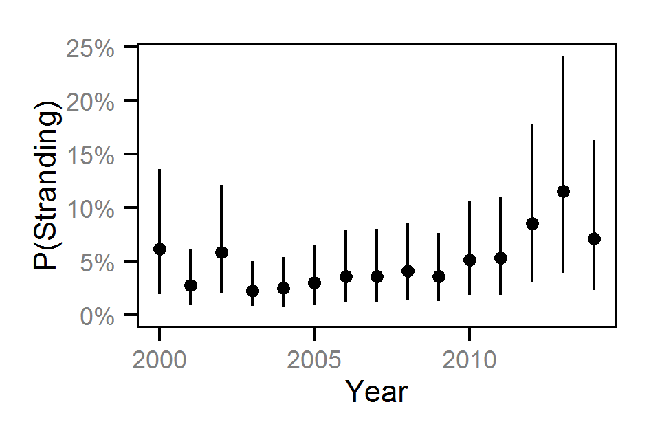
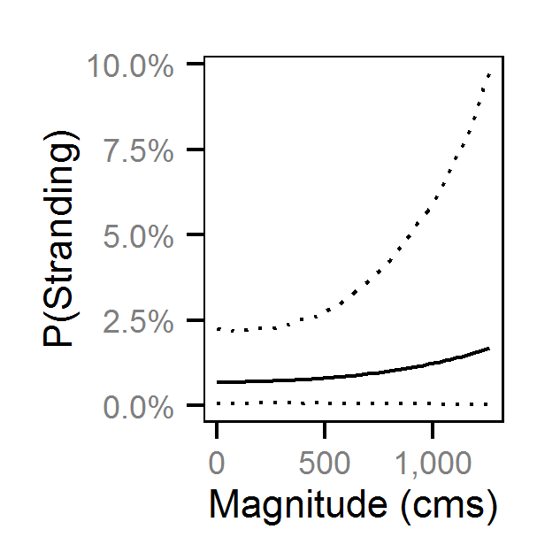
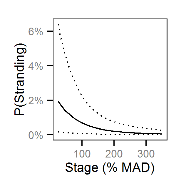
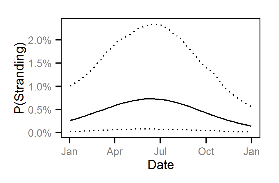
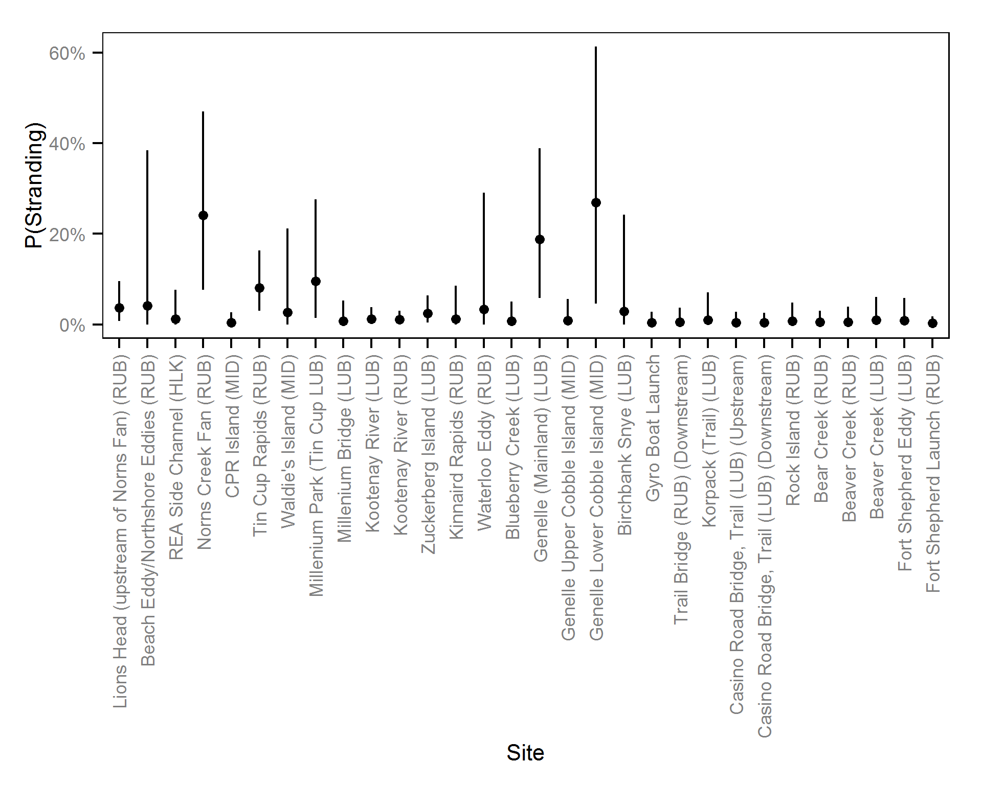
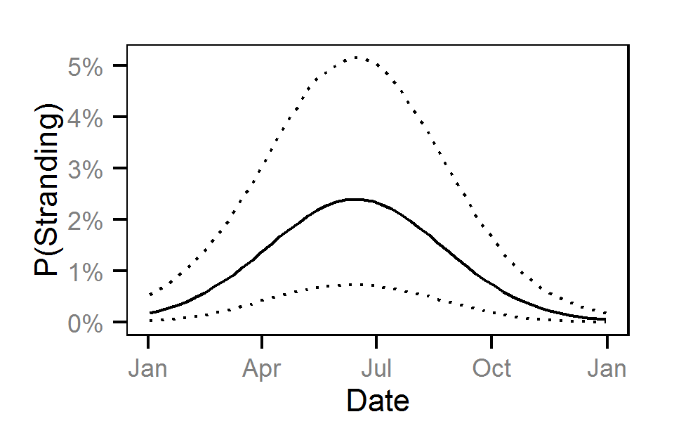
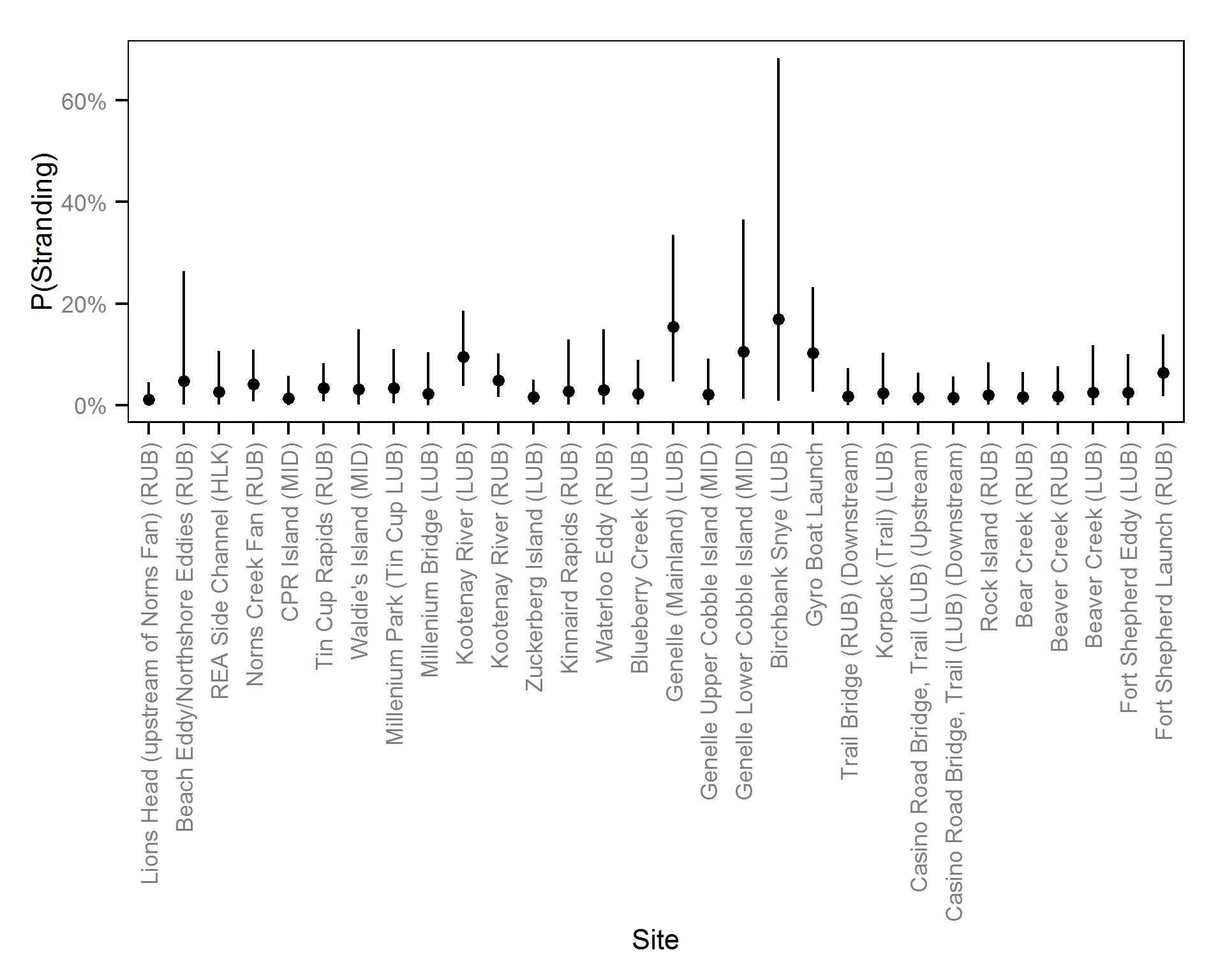
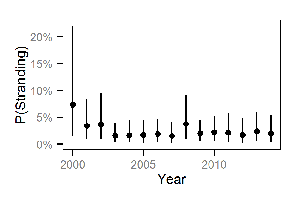
The results are displayed graphically by plotting the modeled relationships between particular variables and the response with 95% credible intervals (CRIs) with the remaining variables held constant. In general, continuous and discrete fixed variables are held constant at their mean and first level values respectively while random variables are held constant at their typical values (expected values of the underlying hyperdistributions) (Kéry and Schaub, 2011, pp. 77-82). Where informative the influence of particular variables is expressed in terms of the effect size (i.e., percent change in the response variable) with 95% CRIs (Bradford et al. 2005). Plots were produced using the ggplot2 R package (Wickham, 2009).
Pool Stranding
The probability of stranding a threshold number of fish was analysed using a hierarchical Bayesian general linear mixed model (GLMM) (Kéry and Schaub, 2011, pp. 73-74).
Key assumptions of the GLMM include:
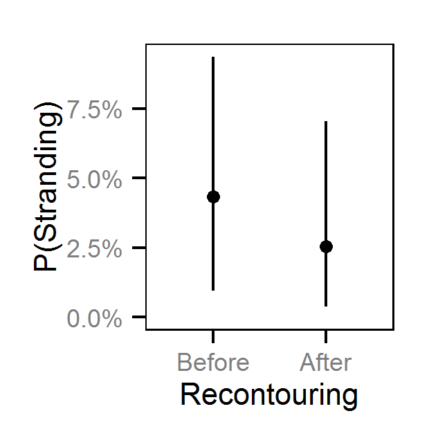
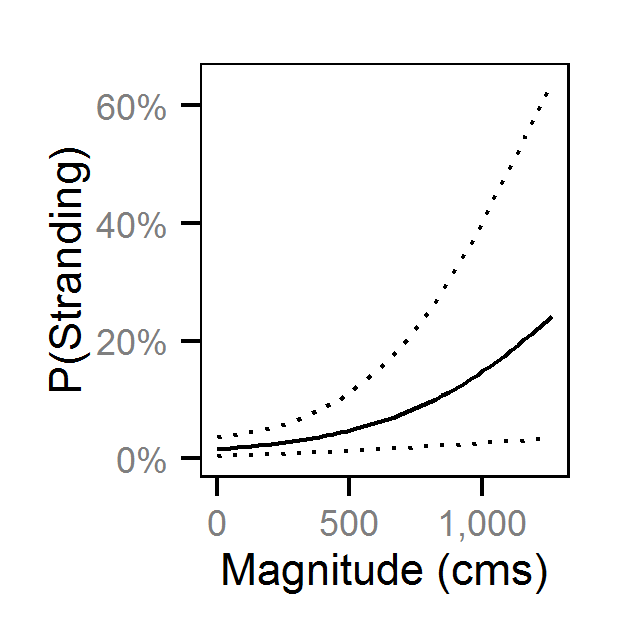
- The probability of stranding varies with the magnitude of the reduction, the stage, whether a site has been recontoured and the day of the year as a second order polynomial.
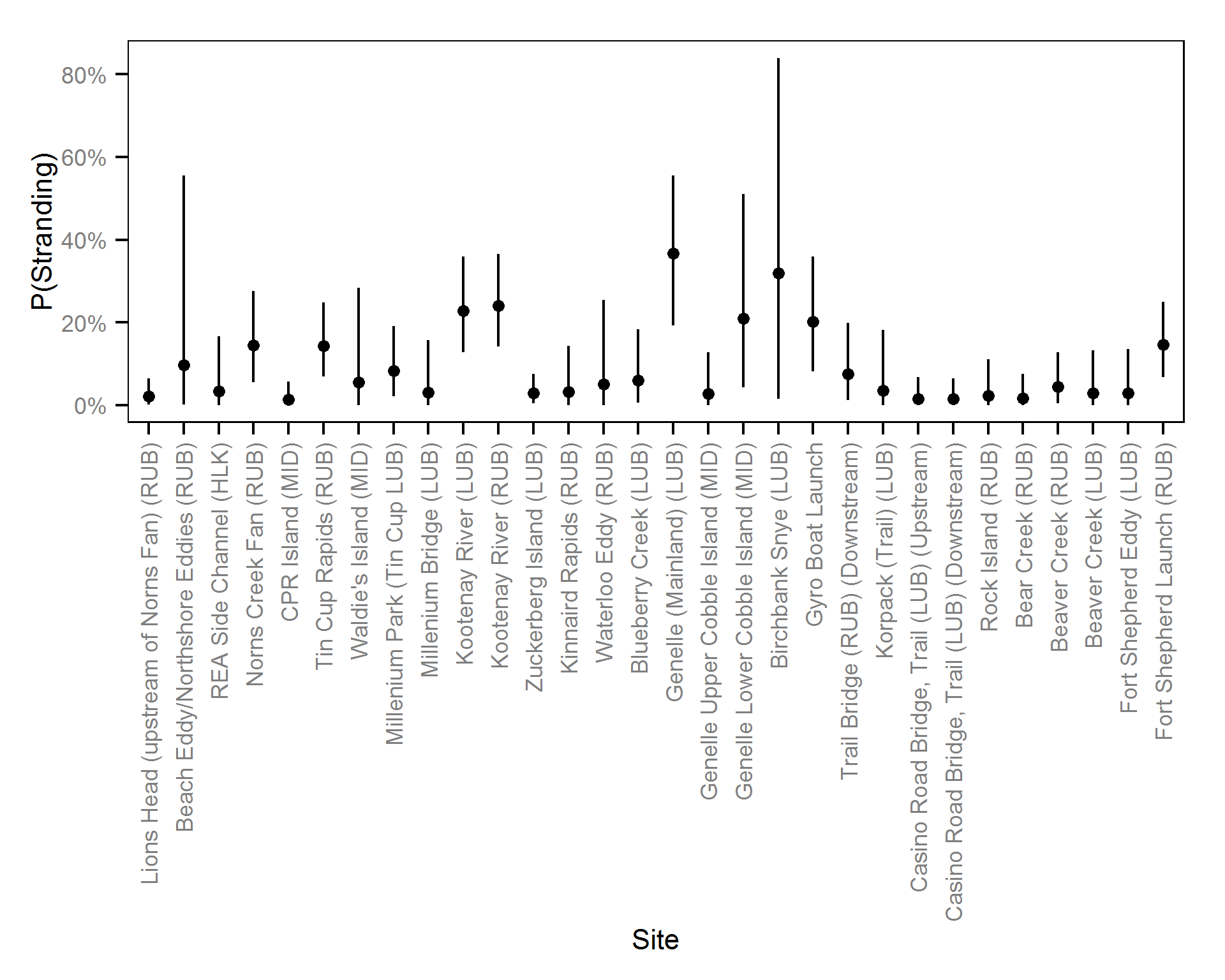
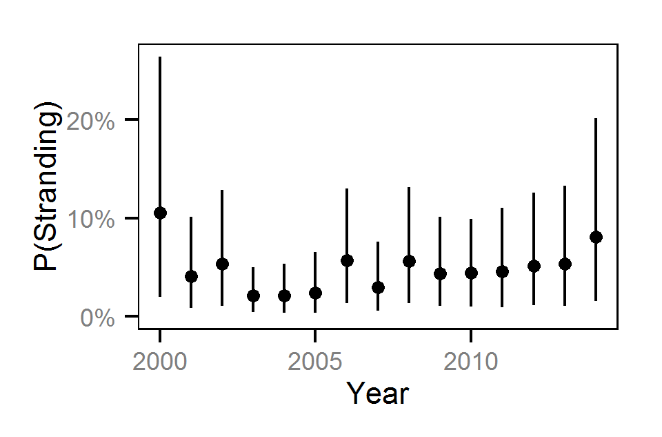
- The probability of stranding can vary randomly with the site and year.
- Stranding events are Bernoulli distributed
Preliminary analysis indicated that the data were not overdispersed. Preliminary analysis also indicated that the rate of reduction, the delay between the reduction and salvage and the diel period were not informative predictors of the probability of stranding.
Model Code
The JAGS model code, which uses a series of naming conventions, is presented below.
Pool Stranding
| Variable/Parameter | Description |
|---|---|
bStranding |
Intercept for logit(eStranding) |
bStrandingDayte |
Effect of Dayte on logit(eStranding) |
bStrandingDayte2 |
Quadratic effect of Dayte on logit(eStranding) |
bStrandingMagnitude |
Effect of Magnitude on logit(eStranding) |
bStrandingRecontoured |
Effect of Recontoured on logit(eStranding) |
bStrandingStage |
Effect of Stage on logit(eStranding) |
Dayte[i] |
Standardised day of the year for the ith site visit |
eStranding[i] |
Expected probability of a stranding event for the ith site visit |
Magnitude[i] |
Standardised magnitude of the reduction for the ith site visit |
Recontoured[i] |
Whether the site of the ith site had been recontoured |
Site[i] |
Site of the ith site visit |
sStrandingSite |
SD of effect of Site on logit(eStranding) |
sStrandingYear |
SD of effect of Year on logit(eStranding) |
Stage[i] |
Standardised stage of the reduction for the ith site visit |
Stranding[i] |
Whether there was a stranding event for the ith site visit |
Year[i] |
Year of the ith site visit |
Pool Stranding - Model1
model{

  bStranding ~ dnorm(0, 5^-2)
  bStrandingMagnitude ~ dnorm(0, 2^-2)

  bStrandingStage ~ dnorm(0, 2^-2)

  bStrandingDayte ~ dnorm(0, 2^-2)
  bStrandingDayte2 ~ dnorm(0, 2^-2)

  bStrandingRecontoured[1] <- 0
  for (i in 2:nRecontoured) {
    bStrandingRecontoured[i] ~ dnorm(0, 2^-2)
  }

  sStrandingSite ~ dunif(0, 5)
  for (i in 1:nSite) {
    bStrandingSite[i] ~ dnorm(0, sStrandingSite^-2)
  }

  sStrandingYear ~ dunif(0, 5)
  for (i in 1:nYear) {
    bStrandingYear[i] ~ dnorm(0, sStrandingYear^-2)
  }

  for(i in 1:length(Stranding)) {

    logit(eStranding[i]) <- bStranding + bStrandingMagnitude * Magnitude[i] + bStrandingStage * Stage[i] + bStrandingDayte * Dayte[i] + bStrandingDayte2 * Dayte[i]^2 + bStrandingRecontoured[Recontoured[i]] + bStrandingSite[Site[i]] + bStrandingYear[Year[i]]

    Stranding[i] ~ dbern(eStranding[i])
  }
}
Results
Model Parameters
The posterior distributions for the fixed (Kery and Schaub 2011 p. 75) parameters in each model are summarised below.
Pool Stranding - Sculpin - One Or More
| Parameter | Estimate | Lower | Upper | SD | Error | Significance |
|---|---|---|---|---|---|---|
| bStranding | -3.16066 | -4.1376 | -2.3169 | 0.46753 | 29 | 0.0000 |
| bStrandingDayte | -0.27833 | -0.4405 | -0.1075 | 0.08280 | 60 | 0.0000 |
| bStrandingDayte2 | -0.01394 | -0.2132 | 0.1756 | 0.09815 | 1395 | 0.9093 |
| bStrandingMagnitude | 0.25979 | 0.1164 | 0.3976 | 0.07254 | 54 | 0.0000 |
| bStrandingRecontoured[2] | -1.17882 | -1.8244 | -0.5874 | 0.31787 | 52 | 0.0000 |
| bStrandingStage | -0.62849 | -0.8252 | -0.4379 | 0.09768 | 31 | 0.0000 |
| sStrandingSite | 1.70997 | 1.0933 | 2.7044 | 0.40697 | 47 | 0.0000 |
| sStrandingYear | 0.61514 | 0.3688 | 1.0140 | 0.16176 | 52 | 0.0000 |
| Rhat | Iterations |
|---|---|
| 1.04 | 4000 |
Pool Stranding - Sculpin - Ten Or More
| Parameter | Estimate | Lower | Upper | SD | Error | Significance |
|---|---|---|---|---|---|---|
| bStranding | -5.29866 | -7.2943 | -3.76398 | 0.8906 | 33 | 0.0000 |
| bStrandingDayte | -0.30239 | -0.6545 | 0.04839 | 0.1797 | 116 | 0.0960 |
| bStrandingDayte2 | -0.55314 | -1.0329 | -0.12428 | 0.2310 | 82 | 0.0093 |
| bStrandingMagnitude | 0.03771 | -0.2787 | 0.33702 | 0.1605 | 816 | 0.8040 |
| bStrandingRecontoured[2] | -1.42702 | -2.5061 | -0.34954 | 0.5471 | 76 | 0.0107 |
| bStrandingStage | -0.51754 | -0.8722 | -0.18193 | 0.1742 | 67 | 0.0013 |
| sStrandingSite | 2.68710 | 1.4082 | 4.42674 | 0.7799 | 56 | 0.0000 |
| sStrandingYear | 0.88486 | 0.4123 | 1.51799 | 0.2928 | 62 | 0.0000 |
| Rhat | Iterations |
|---|---|
| 1.07 | 4000 |
Pool Stranding - Dace - One Or More
| Parameter | Estimate | Lower | Upper | SD | Error | Significance |
|---|---|---|---|---|---|---|
| bStranding | -3.2405 | -4.64792 | -2.2710 | 0.59887 | 37 | 0.0000 |
| bStrandingDayte | -0.7207 | -1.00739 | -0.4543 | 0.14410 | 38 | 0.0000 |
| bStrandingDayte2 | -1.1041 | -1.46664 | -0.7673 | 0.18265 | 32 | 0.0000 |
| bStrandingMagnitude | 0.2399 | 0.08096 | 0.4035 | 0.08229 | 67 | 0.0013 |
| bStrandingRecontoured[2] | -0.6503 | -1.42697 | 0.1401 | 0.39908 | 120 | 0.1120 |
| bStrandingStage | -0.3800 | -0.62671 | -0.1641 | 0.11692 | 61 | 0.0000 |
| sStrandingSite | 1.8781 | 1.04138 | 3.1457 | 0.55011 | 56 | 0.0000 |
| sStrandingYear | 0.6460 | 0.29142 | 1.1217 | 0.20903 | 64 | 0.0000 |
| Rhat | Iterations |
|---|---|
| 1.08 | 2000 |
Pool Stranding - Dace - Ten Or More
| Parameter | Estimate | Lower | Upper | SD | Error | Significance |
|---|---|---|---|---|---|---|
| bStranding | -3.9103 | -5.01281 | -2.9947 | 0.5237 | 26 | 0.0000 |
| bStrandingDayte | -0.6542 | -1.11642 | -0.2394 | 0.2242 | 67 | 0.0027 |
| bStrandingDayte2 | -1.2960 | -1.87767 | -0.7912 | 0.2808 | 42 | 0.0000 |
| bStrandingMagnitude | 0.3353 | 0.09034 | 0.5685 | 0.1202 | 71 | 0.0080 |
| bStrandingRecontoured[2] | -0.3395 | -1.44092 | 0.7534 | 0.5785 | 323 | 0.5600 |
| bStrandingStage | -0.7419 | -1.17223 | -0.3517 | 0.2076 | 55 | 0.0000 |
| sStrandingSite | 1.4861 | 0.64940 | 2.6581 | 0.5195 | 68 | 0.0000 |
| sStrandingYear | 0.6774 | 0.15446 | 1.3534 | 0.2991 | 88 | 0.0000 |
| Rhat | Iterations |
|---|---|
| 1.04 | 2000 |
Figures
Fork Length
Pool Stranding - Sculpin - One Or More
Pool Stranding - Sculpin - Ten Or More
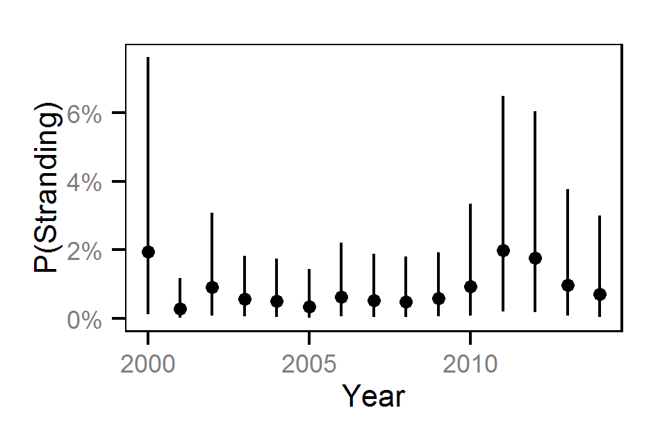
Pool Stranding - Dace - One Or More
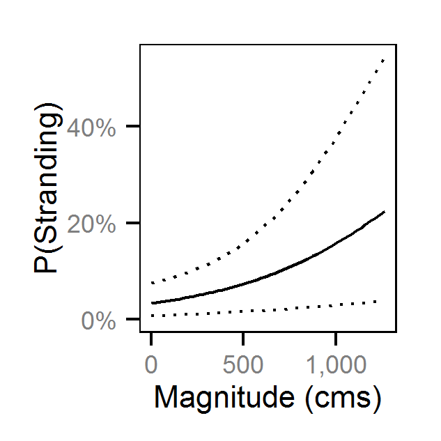
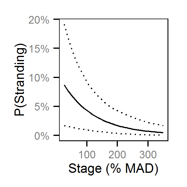
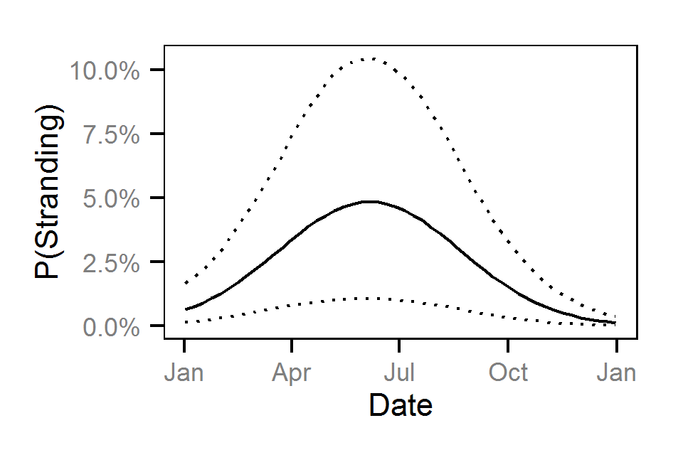
Pool Stranding - Dace - Ten Or More
Acknowledgements
The organisations and individuals whose contributions have made this analysis report possible include:
- BC Hydro
- AMEC Earth and Environmental
- Louise Porto
- Crystal Lawrence
- Golder Associates
- Demitria Burgoon
- Dustin Ford
- Poisson Consulting
- Robyn Irvine
References
- Michael Bradford, Josh Korman, Paul Higgins, (2005) Using confidence intervals to estimate the response of salmon populations (Oncorhynchus spp.) to experimental habitat alterations. Canadian Journal of Fisheries and Aquatic Sciences 62 (12) 2716-2726 10.1139/f05-179
- Hadley Wickham, (2009) ggplot2: elegant graphics for data analysis. http://had.co.nz/ggplot2/book
- Joseph Thorley, (2014) jaggernaut: An R package to facilitate Bayesian analyses using JAGS (Just Another Gibbs Sampler). https://github.com/joethorley/jaggernaut
- Marc Kéry, Michael Schaub, (2011) Bayesian population analysis using {WinBUGS} : a hierarchical perspective. http://www.vogelwarte.ch/bpa.html
- Martyn Plummer, (2012) {JAGS} version 3.3.0 user manual. http://sourceforge.net/projects/mcmc-jags/files/Manuals/3.x/
- R Team, (2013) R: a language and environment for statistical computing. http://www.R-project.org