Middle Columbia River Fish Indexing Analysis 2013
The suggested citation for this analytic report is:
Thorley, J.L. (2015) Middle Columbia River Fish Indexing Analysis 2013. A Poisson Consulting Analysis Report. URL: https://www.poissonconsulting.ca/f/111290438.
Background
The key management questions to be addressed by the analyses are:
- Is there a change in abundance of adult life stages of fish using the Middle Columbia River (MCR) that corresponds with the implementation of a year-round minimum flow?
- Is there a change in growth rate of adult life stages of the most common fish species using the MCR that corresponds with the implementation of a year-round minimum flow?
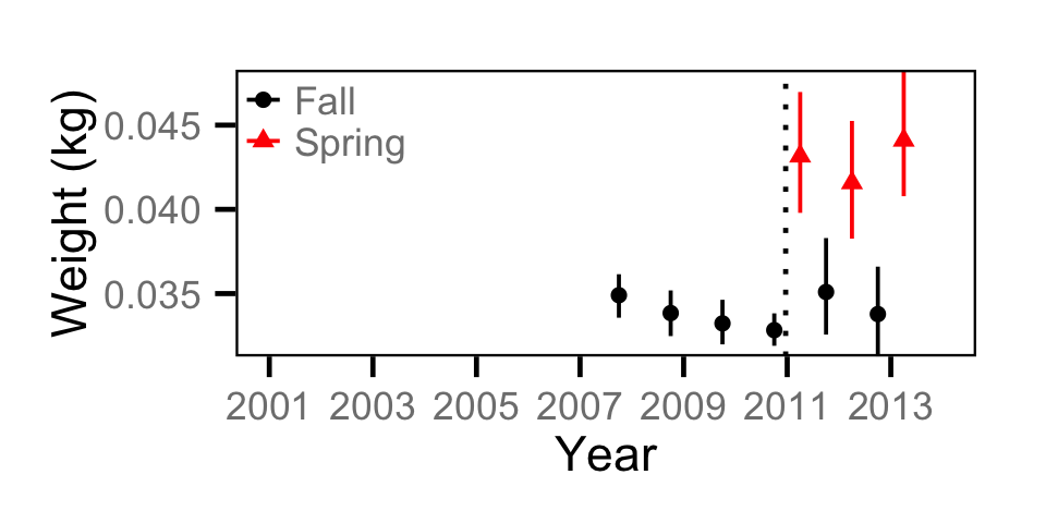
- Is there a change in body condition (measured as a function of relative weight to length) of adult life stages of fish using the MCR that corresponds with the implementation of a year-round minimum flow?
- Is there a change in spatial distribution of adult life stages of fish using the MCR that corresponds with the implementation of a year-round minimum flow?
Other objectives include the estimation of species richness, species diversity (evenness) and biomass and the modeling of environmental-fish metric relationships. The year-round minimum flow was implemented in the winter of 2010 at the same time that a fifth turbine was added.
The data were provided by Golder Associates.
Methods
The four primary fish species were categorized as fry, juvenile or adult based on their lengths.
| Species | Fry | Juvenile |
|---|---|---|
| Bull Trout | < 120 | < 400 |
| Mountain Whitefish | < 120 | < 175 |
| Rainbow Trout | < 120 | < 250 |
| Largescale Sucker | < 350 |
Hierarchical Bayesian models were fitted to the fish indexing data for the MCR using R version 3.0.3 (Team, 2013) and JAGS 3.3.0 (Plummer, 2012) which interfaced with each other via jaggernaut 1.7 (Thorley, 2014). For additional information on hierarchical Bayesian modelling in the BUGS language, of which JAGS uses a dialect, the reader is referred to Kery and Schaub (2011) pages 41-44.
Unless specified, the models assumed vague (low information) prior distributions (Kery and Schaub, 2011, p. 36). The posterior distributions were estimated from a minimum of 1,000 Markov Chain Monte Carlo (MCMC) samples thinned from the second halves of three chains (Kery and Schaub, 2011, pp. 38-40). Model convergence was confirmed by ensuring that Rhat (Kery and Schaub, 2011, p. 40) was less than 1.1 for each of the parameters in the model (Kery and Schaub, 2011, p. 61). Model adequacy was confirmed by examination of residual plots.
The posterior distributions of the fixed (Kery and Schaub 2011 p. 75) parameters are summarised below in terms of a point estimate (mean), lower and upper 95% credibility limits (2.5th and 97.5th percentiles), the standard deviation (SD), percent relative error (half the 95% credibility interval as a percent of the point estimate) and significance (Kery and Schaub, 2011, p. 37,42).
The results are displayed graphically by plotting the modeled relationships between particular variables and the response (with 95% credible intervals) with the remaining variables held constant. In general, continuous and discrete fixed variables are held constant at their mean and first level values respectively while random variables are held constant at their typical values (expected values of the underlying hyperdistributions) (Kery and Schaub, 2011, pp. 77-82). Where informative the influence of particular variables is expressed in terms of the effect size (i.e., percent change in the response variable) with 95% credible intervals (Bradford et al. 2005). Plots were produced using the ggplot2 R package (Wickham, 2009).
Occupancy and Species Richness
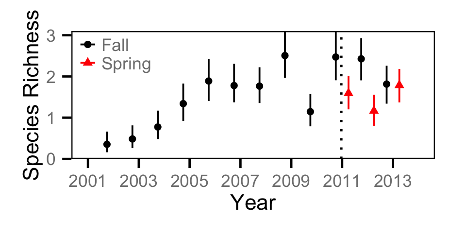
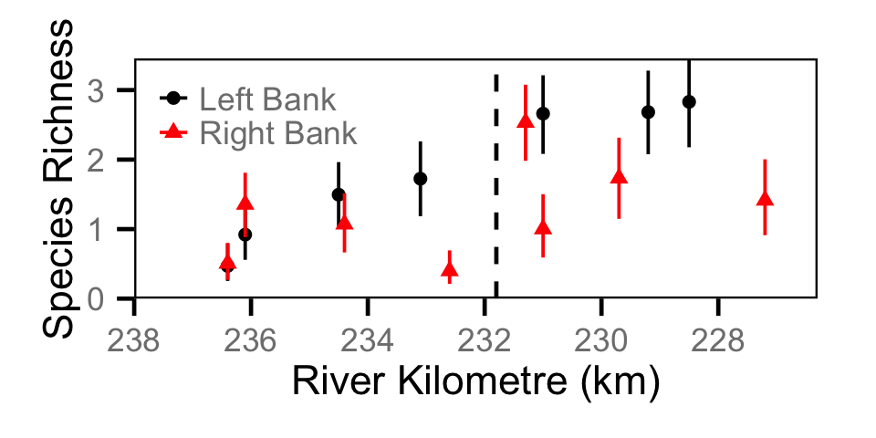
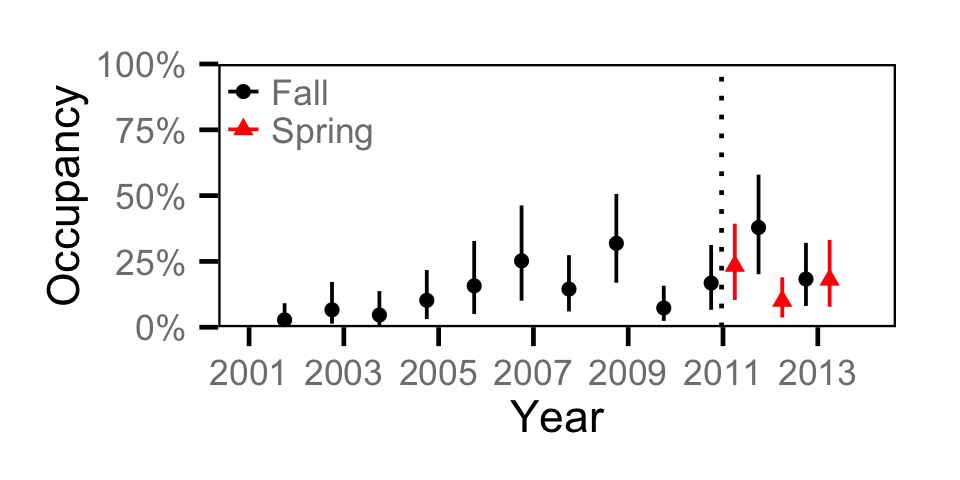
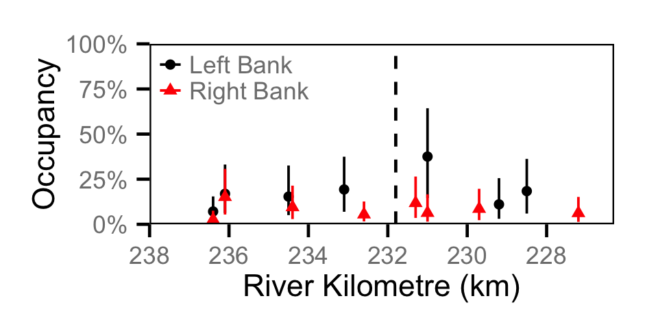
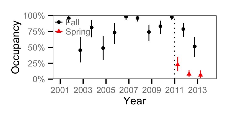
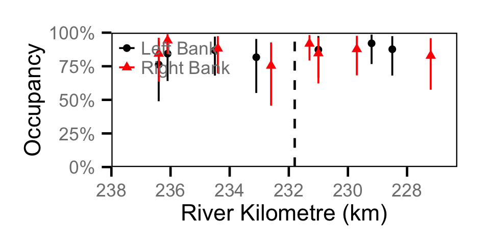
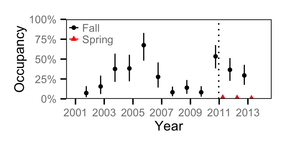
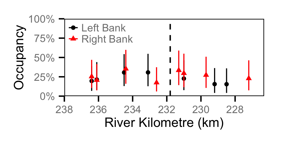
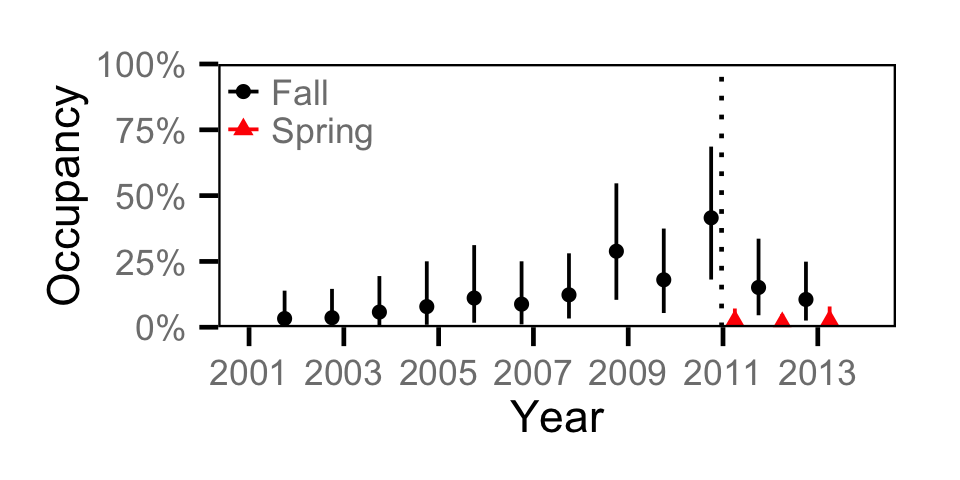
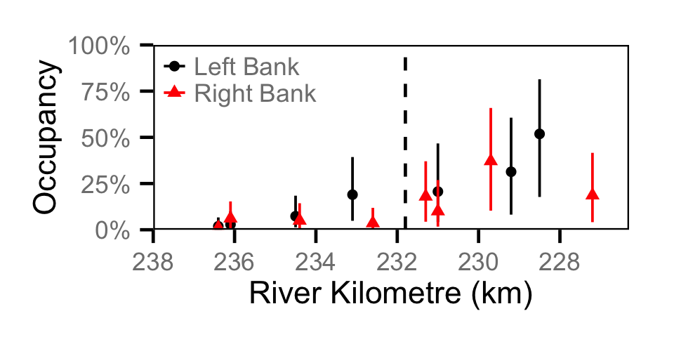
Occupancy which is the probability that a particular species was present at a site was estimated from the temporal replication of detection data (Kery, 2010; Kery and Schaub, 2011, pp. 238-242 and 414-418), i.e., each site was surveyed multiple times within a season. A species was considered to have been detected if one or more individuals of the species were caught or counted. Its important to note that the model estimates the probability that the species was present at a given (or typical) site in a given (or typical) year as opposed to the probability that the species was present in the entire study area. The estimated occupancies for multiple species were summed to give the expected species richnesses.
Key assumptions of the occupancy model include:
- Occupancy (probability of presence) varies with discharge regime and season.
- Occupancy varies randomly with site, year, and the interaction between site and year.
- Sites are closed, i.e., the species is present or absent at a site for all the sessions in a particular season of a year.
- Observed presence is described by a bernoulli distribution.
Count and Species Evenness
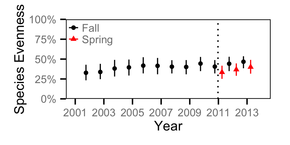
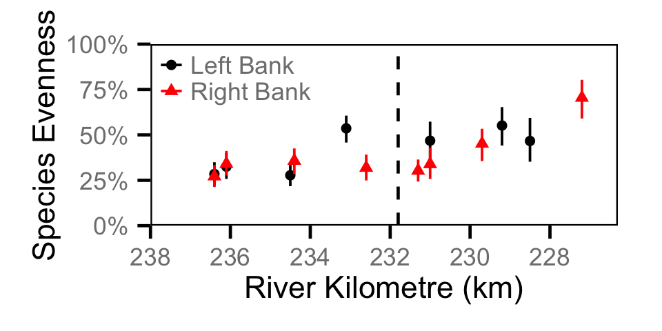
The count data were analysed using an overdispersed Poisson model (Kery, 2010; Kery and Schaub, 2011, pp. 168-170,180 and 55-56). Unlike Kery (2010) and Kery and Schaub (2011), which used a log-normal distribution to account for the extra-Poisson variation, the current model used a gamma distribution with identical shape and scale parameters because it has a mean of 1 and therefore no overall effect on the expected count. The model does not distinguish between the abundance and observer efficiency, i.e., it estimates the count which is the product of the two. As such it is necessary to assume that changes in observer efficiency are negligible in order to interpret the estimates as relative abundance. The shannon index of evenness (\(E\)) was calculated using the following formula where \(S\) is the number of species and \(p_i\) is the proportion of the total count belonging to the ith species.
\[ E = \frac{-\sum p_i \log(p_i)}{ln(S)}\]
Key assumptions of the count model include:
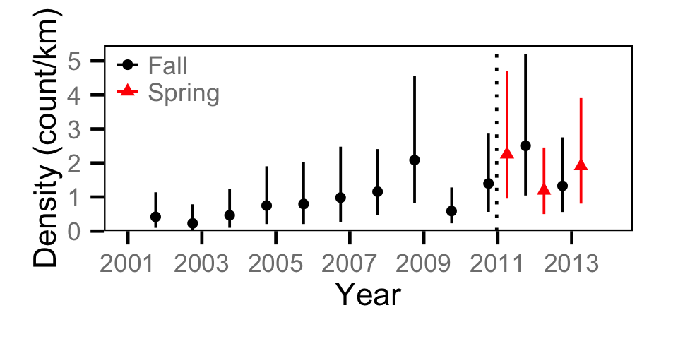
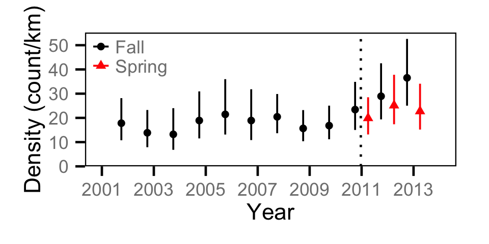
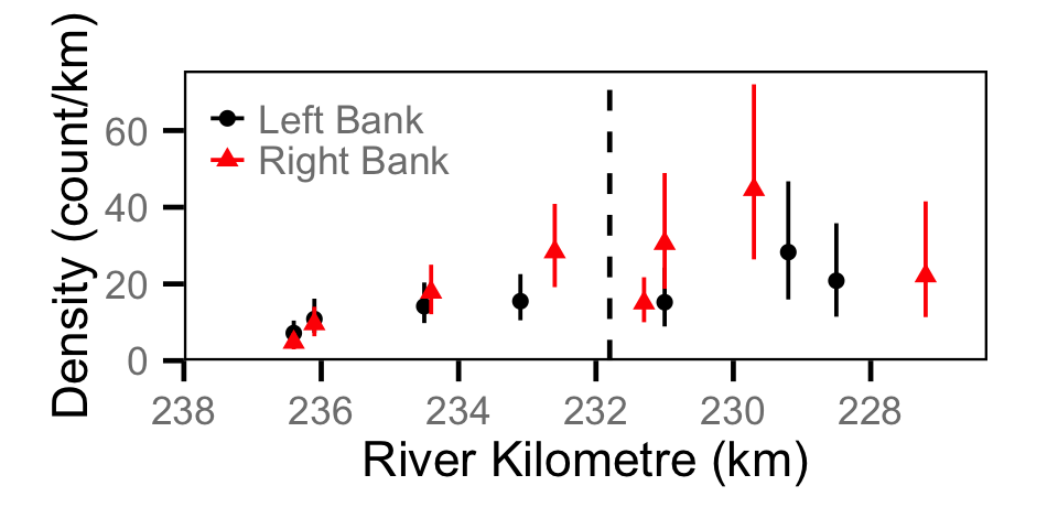
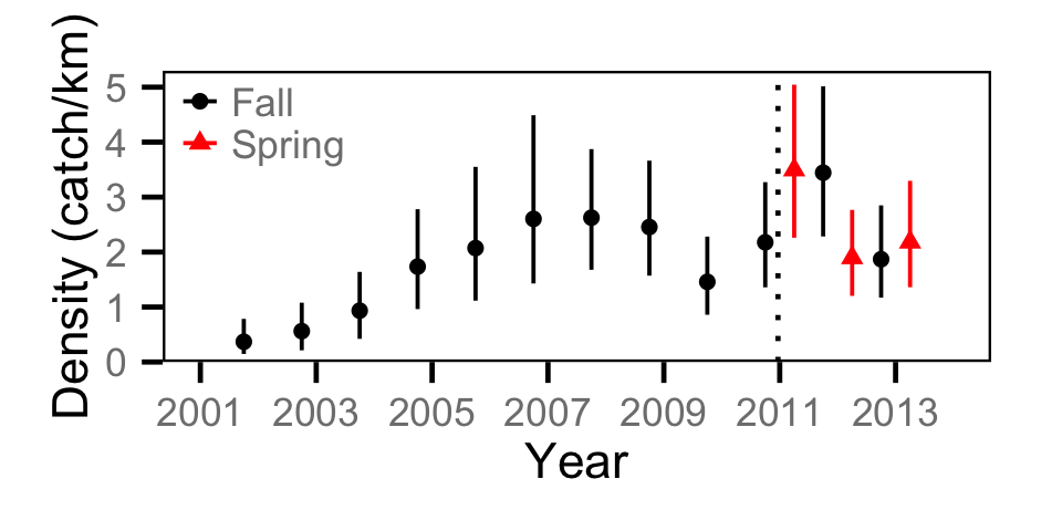
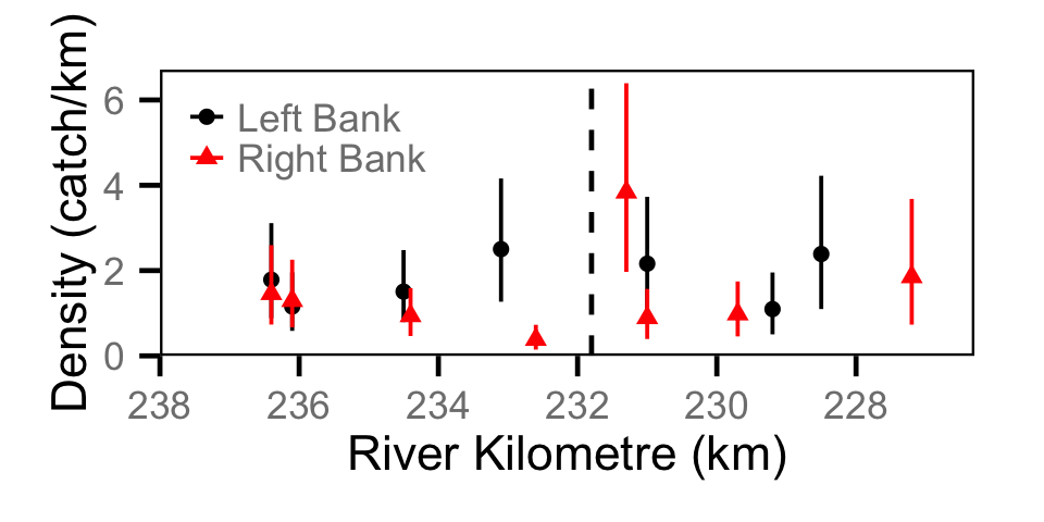
- Count density (count/km) varies with discharge regime, season and river kilometre.
- Count density (count/km) varies randomly with site, year, and the interaction between site and year.
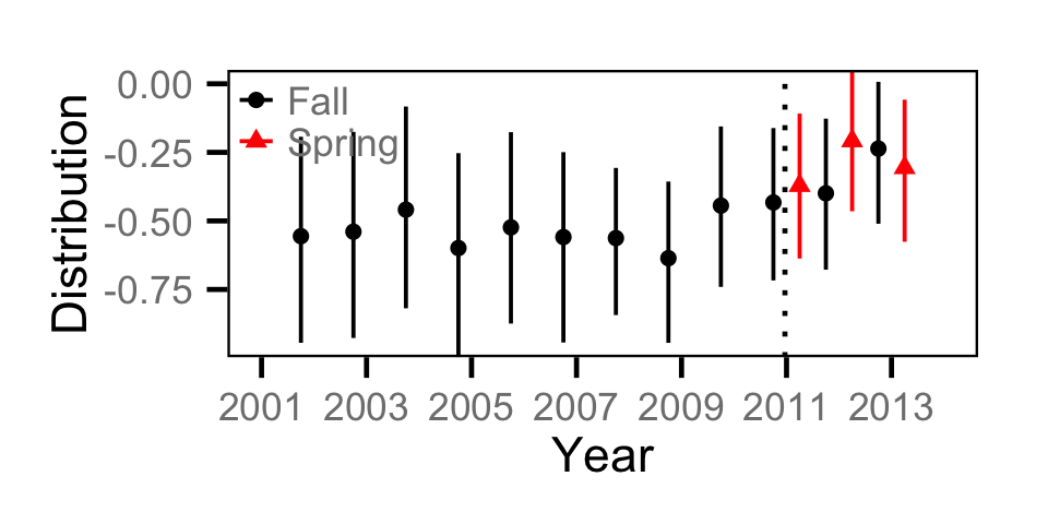
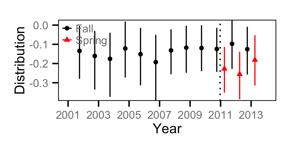
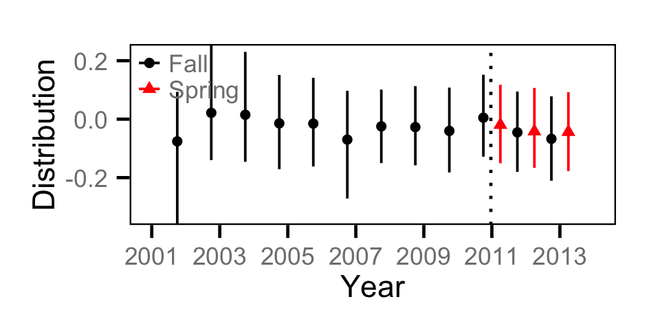
- The relationship between count density and river kilometre (distribution) varies with discharge regime and season.
- The relationship between count density and river kilometre (distribution) varies randomly with year.
- Expected counts are the product of the count density (count/km) and the length of bank sampled.
- Sites are closed, i.e., the predicted count at a site is constant for all the sessions in a particular season of a year.
- Observed counts are described by a Poisson-gamma distribution.
Catch
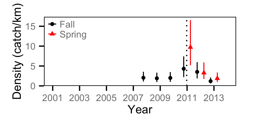
The catch data were analysed using the same overdispersed Poisson model as the count data to provide estimates of relative abundance.
Site Fidelity
The extent to which sites are closed, i.e., fish remain at the same site between sessions, was evaluated from a binomial “t-test” (Kery, 2010, pp. 211-213). The “t-test” estimated the probability that intra-annual recaptures were caught at a different site as previously encountered.
Key assumptions of the site fidelity model include:
- Site fidelity varies with season.
- Observed site fidelity is described by a bernoulli distribution.
Abundance
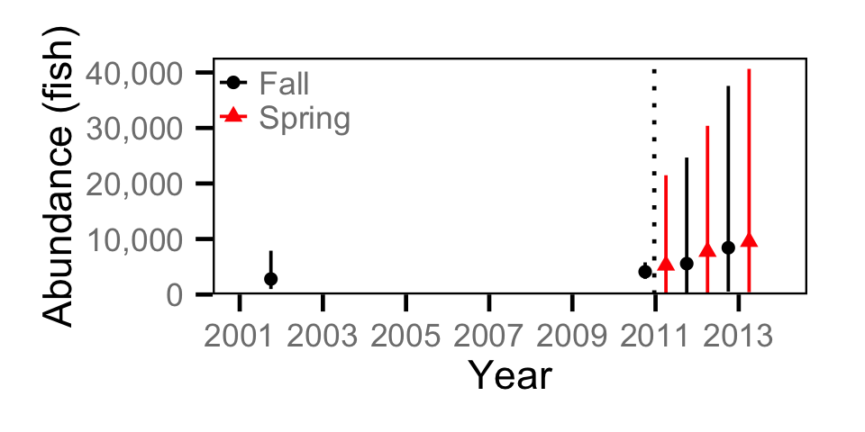
The catch data were also analysed using a capture-recapture-based binomial mixture model (Kery, 2010; Kery and Schaub, 2011, pp. 253-257 and 134-136, 384-388) to provide estimates of capture efficiency and absolute abundance. To maximize the number of recaptures the model grouped all the sites into a supersite for the purposes of estimating the number of marked fish but analysed the total captures at the site level.
Key assumptions of the abundance model include:
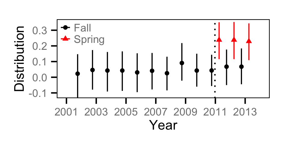
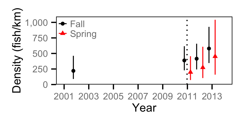
- Lineal density (fish/km) varies with discharge regime, season and river km.
- Lineal density (fish/km) varies randomly with site, year and the interaction between site and year.
- The relationship between density and river kilometre (distribution) varies with discharge regime and season.
- The relationship between density and river kilometre (distribution) varies randomly with year.
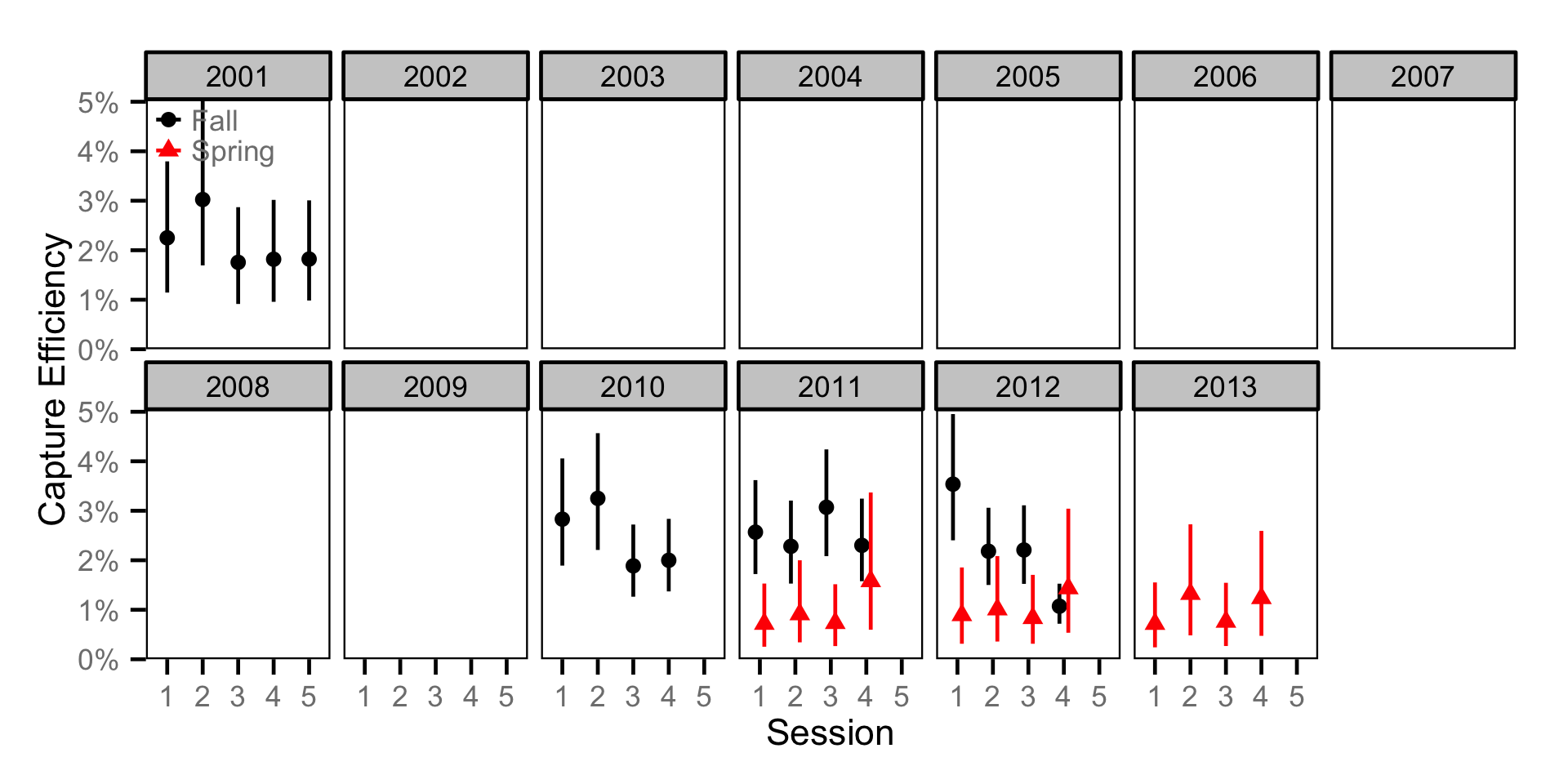
- Efficiency (probability of capture) varies randomly by session within season and year.
- Marked and unmarked fish have the same probability of capture.
- There is no tag loss, mortality or misidentification of fish.
- Sites are closed.
- The number of fish captured are described by binomial distributions.
Capture Efficiency
In order to estimate the capture efficiency independent of abundance a recapture-based binomial model (Kery, 2010; Kery and Schaub, 2011, pp. 253-257 and 134-136,384-388) was fitted to just the marked fish. To maximize the number of recaptures the model grouped all the sites into a supersite.
Key assumptions of the efficiency model include:
- Efficiency (probability of capture) varies randomly by session within season and year.
- There is no tag loss, mortality or misidentification of fish.
- The supersite is closed.
- The number of marked fish caught is described by a binomial distribution.
Growth
Annual growth was estimated from the inter-annual recaptures using the Fabens method (Fabens, 1965) for estimating the von Bertalanffy growth curve (Bertalanffy, 1938).
Key assumptions of the growth model include:
- The growth coefficient varies with discharge regime.
- The growth coefficient varies randomly with year.
- Observed growth (change in length) is normally distributed.
Condition
Condition was estimated via an analysis of weight-length relations (He et al. 2008).
Key assumptions of the condition model include:
- Weight varies with length, discharge regime and season.
- Weight varies randomly with site, year and the interaction between site and year.
- Weight is log-normally distributed.
Length
Mean length was estimated from the measured lengths.
Key assumptions of the length model include:
- Length varies with discharge regime and season.
- Length varies randomly with site, year and the interaction between site and year.
- Length is log-normally distributed.
Biomass
The biomass was calculated from the posterior distributions for the Length, Condition and Abundance analyses.
Multivariate Analyses
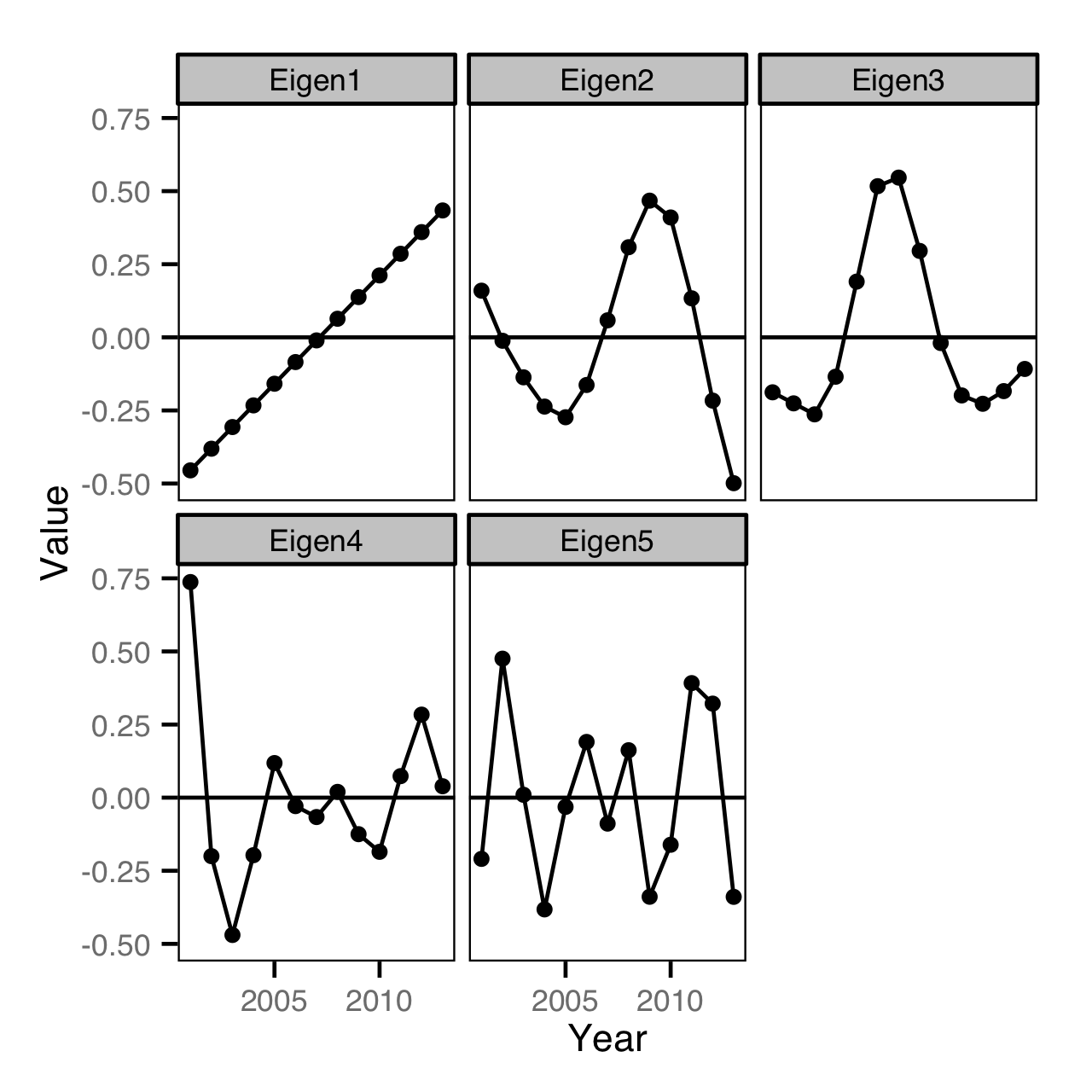
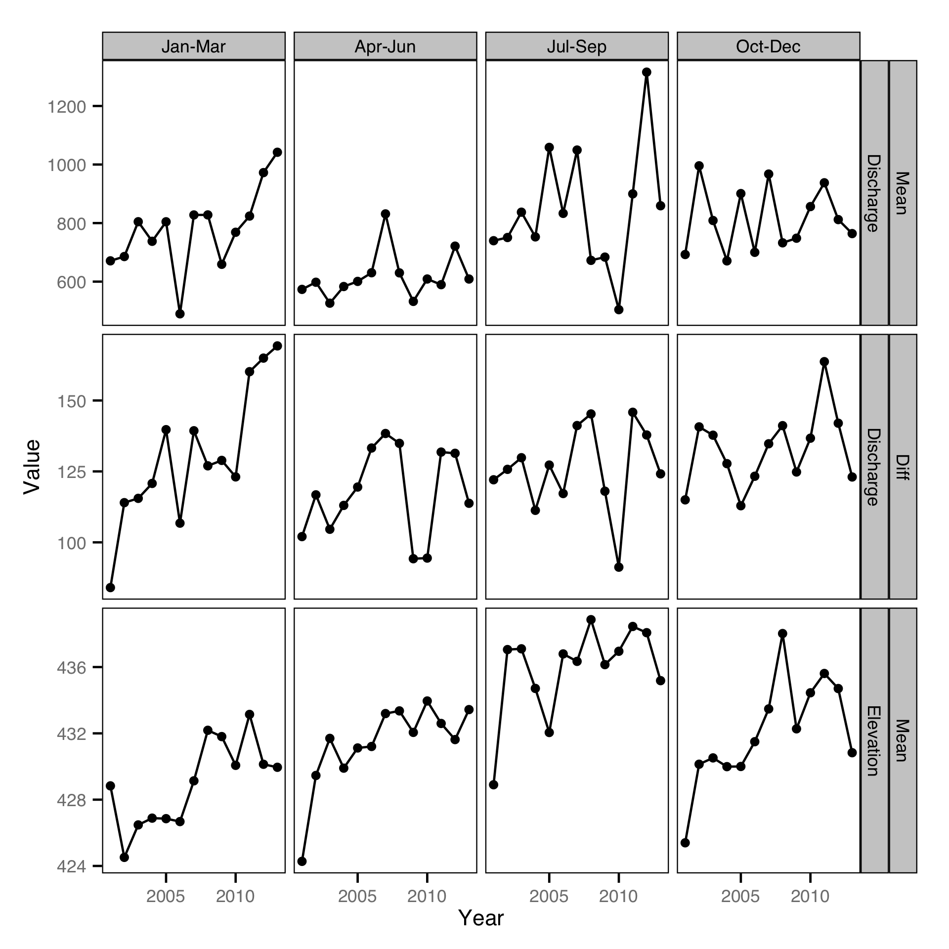
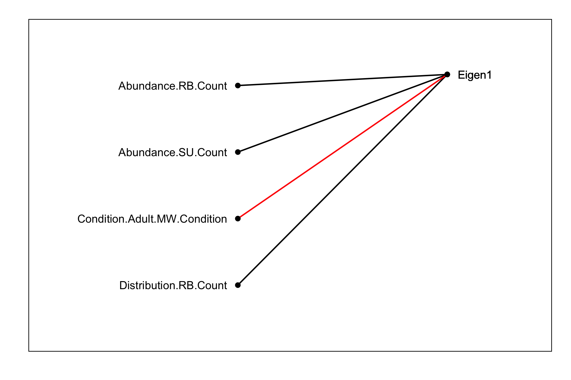
In order to examine the relationships between environmental variables and the fish indexing metrics multivariate analyses were performed. More specifically the trimonthly mean discharge and elevation and the trimonthly mean absolute hourly discharge change were analysed to get their five primary eigenvectors. Next the correlations between the trimonthly environmental time series and the eigenvectors was quantified using a Bayesian model. The same model was also used to quantify the correlations between the eigenvectors and fish indexing time series related to the management hypotheses. Significant relationships were indicated using time series/eigenvector connectivity plots were nodes are connected if the relationship is significant and positive relationships are in black and negative ones in red.
Model Code
The JAGS model code, which uses a series of naming conventions, is presented below.
Occupancy
| Variable/Parameter | Description |
|---|---|
bOccupancy |
Intercept of logit(eOccupancy) |
bOccupancyRegime[i] |
Effect of ith regime on logit(eOccupancy) |
bOccupancySeason[i] |
Effect of ith season on logit(eOccupancy) |
bOccupancySite[i] |
Effect of ith site on logit(eOccupancy) |
bOccupancySiteYear[i, j] |
Effect of ith site in jth year on logit(eOccupancy) |
bOccupancyYear[i] |
Effect of ith year on logit(eOccupancy) |
eObserved[i] |
Predicted probability of observing species on ith site visit |
eOccupancy[i] |
Predicted occupancy (species presence versus absence) on ith site visit |
Observed[i] |
Whether the species was observed on ith site visit |
Occupancy - Model1
model {

  bOccupancy ~ dnorm(0, 5^-2)

  bOccupancySeason[1] <- 0
  for(i in 2:nSeason) {
    bOccupancySeason[i] ~ dnorm(0, 5^-2)
  }

  bOccupancyRegime[1] <- 0
  for(i in 2:nRegime) {
    bOccupancyRegime[i] ~ dnorm(0, 5^-2)
  }

  sOccupancyYear ~ dunif(0, 5)
  for (yr in 1:nYear) {
    bOccupancyYear[yr] ~ dnorm(0, sOccupancyYear^-2)
  }

  sOccupancySite ~ dunif(0, 5)
  sOccupancySiteYear ~ dunif(0, 5)
  for (st in 1:nSite) {
    bOccupancySite[st] ~ dnorm(0, sOccupancySite^-2)
    for (yr in 1:nYear) {
      bOccupancySiteYear[st, yr] ~ dnorm(0, sOccupancySiteYear^-2)
    }
  }

  for (i in 1:length(Year)) {

    logit(eOccupancy[i]) <- bOccupancy
      + bOccupancyRegime[Regime[i]] + bOccupancySeason[Season[i]]
      + bOccupancySite[Site[i]] + bOccupancyYear[Year[i]]
      + bOccupancySiteYear[Site[i],Year[i]]

    eObserved[i] <- eOccupancy[i]

    Observed[i] ~ dbern(eObserved[i])
  }
}
Count
| Variable/Parameter | Description |
|---|---|
bDensity |
Intercept of log(eDensity) |
bDensityRegime[i] |
Effect of ith regime on log(eDensity) |
bDensitySeason[i] |
Effect of ith season on log(eDensity) |
bDensitySite[i] |
Effect of ith site on log(eDensity) |
bDensitySiteYear[i, j] |
Effect of ith site in jth year on log(eDensity) |
bDensityYear[i] |
Effect of ith year on log(eDensity) |
bDispersion |
Overdispersion parameter |
bDistribution |
Intercept of eDistribution |
bDistributionRegime[i] |
Effect of ith regime on eDistribution |
bDistributionSeason[i] |
Effect of ith season on eDistribution |
bDistributionYear[i] |
Effect of ith year on eDistribution |
Count[i] |
Count on ith site visit |
eCount[i] |
Predicted count on ith site visit |
eDensity[i] |
Predicted lineal count density on ith site visit |
eDispersion[i] |
Predicted dispersion on ith site visit |
eDistribution[i] |
Predicted effect of centred river kilometre on ith site visit on log(eDensity) |
Count - Model1
model {

  bDensity ~ dnorm(0, 5^-2)
  bDistribution ~ dnorm(0, 5^-2)

  bDensityRegime[1] <- 0
  bDistributionRegime[1] <- 0
  for(i in 2:nRegime) {
    bDensityRegime[i] ~ dnorm(0, 5^-2)
    bDistributionRegime[i] ~ dnorm(0, 5^-2)
  }

  bDensitySeason[1] <- 0
  bDistributionSeason[1] <- 0
  for(i in 2:nSeason) {
    bDensitySeason[i] ~ dnorm(0, 5^-2)
    bDistributionSeason[i] ~ dnorm(0, 5^-2)
  }

  sDensityYear ~ dunif(0, 2)
  sDistributionYear ~ dunif(0, 2)
  for (i in 1:nYear) {
    bDensityYear[i] ~ dnorm(0, sDensityYear^-2)
    bDistributionYear[i] ~ dnorm(0, sDistributionYear^-2)
  }

  sDensitySite ~ dunif(0, 5)
  sDensitySiteYear ~ dunif(0, 2)
  for (i in 1:nSite) {
    bDensitySite[i] ~ dnorm(0, sDensitySite^-2)
    for (j in 1:nYear) {
      bDensitySiteYear[i, j] ~ dnorm(0, sDensitySiteYear^-2)
    }
  }

  bDispersion ~ dgamma(0.1, 0.1)

  for (i in 1:length(Year)) {

      eDistribution[i] <- bDistribution
      + bDistributionRegime[Regime[i]] + bDistributionSeason[Season[i]]
      + bDistributionYear[Year[i]]

    log(eDensity[i]) <- bDensity
      + eDistribution[i] * RiverKm[i]
      + bDensityRegime[Regime[i]] + bDensitySeason[Season[i]]
      + bDensitySite[Site[i]] + bDensityYear[Year[i]]
      + bDensitySiteYear[Site[i],Year[i]]

    eCount[i] <- eDensity[i] * SiteLength[i] * ProportionSampled[i]

    eDispersion[i] ~ dgamma(bDispersion, bDispersion)

    Count[i] ~ dpois(eCount[i] * eDispersion[i])
  }
  tAbundance <- bDensityRegime[2]
  tDistribution <- bDistributionRegime[2]
}
Catch
| Variable/Parameter | Description |
|---|---|
bDensity |
Intercept of log(eDensity) |
bDensityRegime[i] |
Effect of ith regime on log(eDensity) |
bDensitySeason[i] |
Effect of ith season on log(eDensity) |
bDensitySite[i] |
Effect of ith site on log(eDensity) |
bDensitySiteYear[i, j] |
Effect of ith site in jth year on log(eDensity) |
bDensityYear[i] |
Effect of ith year on log(eDensity) |
bDispersion |
Overdispersion parameter |
bDistribution |
Intercept of eDistribution |
bDistributionRegime[i] |
Effect of ith regime on eDistribution |
bDistributionSeason[i] |
Effect of ith season on eDistribution |
bDistributionYear[i] |
Effect of ith year on eDistribution |
Catch[i] |
Catch on ith site visit |
eCatch[i] |
Predicted catch on ith site visit |
eDensity[i] |
Predicted lineal catch density on ith site visit |
eDispersion[i] |
Predicted dispersion on ith site visit |
eDistribution[i] |
Predicted effect of centred river kilometre on ith site visit on log(eDensity) |
Catch - Model1
model {

  bDensity ~ dnorm(0, 5^-2)
  bDistribution ~ dnorm(0, 5^-2)

  bDensityRegime[1] <- 0
  bDistributionRegime[1] <- 0
  for(i in 2:nRegime) {
    bDensityRegime[i] ~ dnorm(0, 5^-2)
    bDistributionRegime[i] ~ dnorm(0, 5^-2)
  }

  bDensitySeason[1] <- 0
  bDistributionSeason[1] <- 0
  for(i in 2:nSeason) {
    bDensitySeason[i] ~ dnorm(0, 5^-2)
    bDistributionSeason[i] ~ dnorm(0, 5^-2)
  }

  sDensityYear ~ dunif(0, 2)
  sDistributionYear ~ dunif(0, 2)
  for (i in 1:nYear) {
    bDensityYear[i] ~ dnorm(0, sDensityYear^-2)
    bDistributionYear[i] ~ dnorm(0, sDistributionYear^-2)
  }

  sDensitySite ~ dunif(0, 5)
  sDensitySiteYear ~ dunif(0, 2)
  for (i in 1:nSite) {
    bDensitySite[i] ~ dnorm(0, sDensitySite^-2)
    for (j in 1:nYear) {
      bDensitySiteYear[i, j] ~ dnorm(0, sDensitySiteYear^-2)
    }
  }

  bDispersion ~ dgamma(0.1, 0.1)

  for (i in 1:length(Year)) {
    eDistribution[i] <- bDistribution
      + bDistributionRegime[Regime[i]]
      + bDistributionSeason[Season[i]]
      + bDistributionYear[Year[i]]

    log(eDensity[i]) <- bDensity
      + eDistribution[i] * RiverKm[i]
      + bDensityRegime[Regime[i]] + bDensitySeason[Season[i]]
      + bDensitySite[Site[i]] + bDensityYear[Year[i]]
      + bDensitySiteYear[Site[i],Year[i]]

    eCatch[i] <- eDensity[i] * SiteLength[i] * ProportionSampled[i]

    eDispersion[i] ~ dgamma(bDispersion, bDispersion)

    Catch[i] ~ dpois(eCatch[i] * eDispersion[i])
  }
  tAbundance <- bDensityRegime[2]
  tDistribution <- bDistributionRegime[2]
}
Site Fidelity
| Variable/Parameter | Description |
|---|---|
| bMoved | Intercept for logit(eMoved) |
| bMovedSeason[i] | Effect of ith season on logit(eMoved) |
| eMoved[i] | Predicted probability of different site for ith recapture |
| Moved[i] | Was ith recapture recorded at a different site as previously encountered |
Site Fidelity - Model1
model {
  bMoved ~ dnorm(0, 5^-2)

  bMovedSeason[1] <- 0
  for(i in 2:nSeason) {
    bMovedSeason[i] ~ dnorm(0, 5^-2)
  }

  for (i in 1:length(Season)) {

    logit(eMoved[i]) <- bMoved + bMovedSeason[Season[i]]

    Moved[i] ~ dbern(eMoved[i])
  }
}
Abundance
| Variable/Parameter | Description |
|---|---|
bDensity |
Intercept for log(eDensity) |
bDensityRegime[i] |
Effect of ith regime on log(eDensity) |
bDensitySeason[i] |
Effect of ith season on log(eDensity) |
bDensitySite[i] |
Effect of ith site on log(eDensity) |
bDensitySiteYear[i, j] |
Effect of ith site in jth year on log(eDensity) |
bDensityYear[i] |
Effect of ith year on log(eDensity) |
bDistribution |
Intercept for eDistribution |
bDistributionRegime[i] |
Effect of ith regime on eDistribution |
bDistributionSeason[i] |
Effect of ith season on eDistribution |
bDistributionYear[i] |
Effect of ith year on eDistribution |
bEfficiency |
Intercept for logit(eEfficiency) |
bEfficiencySessionSeasonYear[i, j, k] |
Effect of ith session in jth season of kth year on logit(eEfficiency) |
Catch[i] |
Number of fish caught on ith site visit |
eAbundance[i] |
Predicted abundance on ith site visit |
eDensity[i] |
Predicted lineal density on ith site visit |
eDistribution[i] |
Predicted effect of centred river kilometre on ith site visit on log(eDensity) |
eEfficiency[i] |
Predicted efficiency during ith site visit |
Marked[i] |
Number of marked fish caught in ith river visit |
Tagged[i] |
Number of fish tagged prior to ith river visit |
Abundance - Model1
model {

  bEfficiency ~ dnorm(0, 5^-2)
  bDensity ~ dnorm(0, 5^-2)
  bDistribution ~ dnorm(0, 5^-2)

  bDensityRegime[1] <- 0
  bDistributionRegime[1] <- 0
  for(i in 2:nRegime) {
    bDensityRegime[i] ~ dnorm(0, 5^-2)
    bDistributionRegime[i] ~ dnorm(0, 5^-2)
  }

  bEfficiencySeason[1] <- 0
  bDensitySeason[1] <- 0
  bDistributionSeason[1] <- 0
  for(i in 2:nSeason) {
    bEfficiencySeason[i] ~ dnorm(0, 5^-2)
    bDensitySeason[i] ~ dnorm(0, 5^-2)
    bDistributionSeason[i] ~ dnorm(0, 5^-2)
  }

  sDensityYear ~ dunif(0, 2)
  sDistributionYear ~ dunif(0, 2)
  for (i in 1:nYear) {
    bDensityYear[i] ~ dnorm(0, sDensityYear^-2)
    bDistributionYear[i] ~ dnorm(0, sDistributionYear^-2)
  }

  sDensitySite ~ dunif(0, 5)
  sDensitySiteYear ~ dunif(0, 2)
  for (i in 1:nSite) {
    bDensitySite[i] ~ dnorm(0, sDensitySite^-2)
    for (j in 1:nYear) {
      bDensitySiteYear[i, j] ~ dnorm(0, sDensitySiteYear^-2)
    }
  }

  sEfficiencySessionSeasonYear ~ dunif(0, 5)
  for (i in 1:nSession) {
    for (j in 1:nSeason) {
      for (k in 1:nYear) {
        bEfficiencySessionSeasonYear[i, j, k] ~ dnorm(0, sEfficiencySessionSeasonYear^-2)
      }
    }
  }

  for(i in 1:length(EffIndex)) {

    logit(eEff[i]) <- bEfficiency
        + bEfficiencySeason[Season[EffIndex[i]]]
        + bEfficiencySessionSeasonYear[Session[EffIndex[i]],
                                       Season[EffIndex[i]],
                                       Year[EffIndex[i]]]

    Marked[EffIndex[i]] ~ dbin(eEff[i], Tagged[EffIndex[i]])
  }

  for (i in 1:length(Year)) {

    logit(eEfficiency[i]) <- bEfficiency
        + bEfficiencySeason[Season[i]]
        + bEfficiencySessionSeasonYear[Session[i], Season[i], Year[i]]

    eDistribution[i] <- bDistribution
      + bDistributionRegime[Regime[i]]
      + bDistributionSeason[Season[i]]
      + bDistributionYear[Year[i]]

    log(eDensity[i]) <- bDensity
      + eDistribution[i] * RiverKm[i]
      + bDensityRegime[Regime[i]]
      + bDensitySeason[Season[i]]
      + bDensitySite[Site[i]]
      + bDensityYear[Year[i]]
      + bDensitySiteYear[Site[i], Year[i]]

    eSamplingEfficiency[i] <- min(eEfficiency[i] * ProportionSampled[i], 0.9)

    eAbundance[i] <- max(round(eDensity[i] * SiteLength[i]), MinAbundance[i])

    Catch[i] ~ dbin(eSamplingEfficiency[i], eAbundance[i])
  }
  tAbundance <- bDensityRegime[2]
  tDistribution <- bDistributionRegime[2]
}
Capture Efficiency
| Variable/Parameter | Description |
|---|---|
bEFficiency |
Intercept of logit(eEfficiency) |
bEFficiencySeason[i] |
Effect of ith season on logit(eEfficiency) |
bEFficiencySessionSeasonYear[i, j, k] |
Effect of ith session within jth season and kth year on logit(eEfficiency) |
eEfficiency[i] |
Predicted efficiency during ith vist |
Marked[i] |
Number of marked fish recaught during ith visit |
Tagged[i] |
Number of marked fish tagged prior to ith visit |
Capture Efficiency - Model1
model {

  bEfficiency ~ dnorm(0, 5^-2)

  bEfficiencySeason[1] <- 0
  for (i in 2:nSeason) {
    bEfficiencySeason[i] ~ dnorm(0, 5^-2)
  }

  sEfficiencySessionSeasonYear ~ dunif(0, 5)
  for (i in 1:nSession) {
    for (j in 1:nSeason) {
      for (k in 1:nYear) {
        bEfficiencySessionSeasonYear[i, j, k] ~ dnorm(0, sEfficiencySessionSeasonYear^-2)
      }
    }
  }

  for(i in 1:length(Year)) {
    logit(eEfficiency[i]) <- bEfficiency
        + bEfficiencySeason[Season[i]]
        + bEfficiencySessionSeasonYear[Session[i], Season[i], Year[i]]

    Marked[i] ~ dbin(eEfficiency[i], Tagged[i])
  }
}
Growth
| Variable/Parameter | Description |
|---|---|
| bK | Intercept of log(eK) |
| bKRegime[i] | Effect of ith regime on log(eK) |
| bKYear[i] | Effect of ith year on log(eK) |
| bLinf | Mean maximum length (von Bertalanffy length-at-infinity) |
| eGrowth[i] | Predicted growth (change in length) of the ith recapture between release and recapture |
| eK[i] | Predicted von Bertalanffy growth coefficient for ith year |
| Growth[i] | Growth (change in length) of the ith recapture between release and recapture |
| LengthAtRelease[i] | Length of the ith recapture when released in a previous year |
| sGrowth | SD of residual variation in Growth |
| Year[i] | Year the ith recapture was released |
| Years[i] | Number of years between release and recapture for the ith recapture |
Growth - Model1
model {

  bK ~ dnorm (0, 5^-2)

  bKRegime[1] <- 0
  for(i in 2:nThreshold) {
    bKRegime[i] ~ dunif(-100, 100)
  }

  sKYear ~ dunif (0, 5)
  for (i in 1:nYear) {
    bKYear[i] ~ dnorm(0, sKYear^-2)
    log(eK[i]) <- bK + bKRegime[step(i - Threshold) + 1] + bKYear[i]
  }

  bLinf ~ dunif(100, 1000)
  sGrowth ~ dunif(0, 100)

  for (i in 1:length(Year)) {
    eGrowth[i] <- (bLinf - LengthAtRelease[i])
                  * (1 - exp(-sum(eK[Year[i]:(Year[i] + Years[i] - 1)])))

    Growth[i] ~ dnorm(eGrowth[i], sGrowth^-2)
  }
  tGrowth <-  bKRegime[2]
}
Condition
| Variable/Parameter | Description |
|---|---|
bWeight |
Intercept for eWeightSlope |
bWeightLength |
Intercept for eWeightIntercept |
bWeightRegime[i] |
Effect of ith regime on eWeightIntercept |
bWeightSeason[i] |
Effect of ith season on eWeightIntercept |
bWeightSite[i] |
Effect of ith site on eWeightIntercept |
bWeightSiteYear[i] |
Effect of ith site in jth year on eWeightIntercept |
bWeightYear[i] |
Effect of ith year on eWeightIntercept |
eWeightIntercept[i] |
Predicted intercept for log(eWeight) |
eWeightSlope[i] |
Predicted effect of centred log length on log(eWeight) |
sWeight |
SD of residual variation in log(Weight) |
Weight[i] |
Weight of ith fish |
Condition - Model1
model {

  bWeight ~ dnorm(5, 5^-2)
  bWeightLength ~ dnorm(3, 5^-2)

  bWeightRegime[1] <- 0
  for(i in 2:nRegime) {
    bWeightRegime[i] ~ dnorm(0, 5^-2)
  }

  bWeightSeason[1] <- 0
  for(i in 2:nSeason) {
    bWeightSeason[i] ~ dnorm(0, 5^-2)
  }

  sWeightYear ~ dunif(0, 5)
  for(yr in 1:nYear) {
    bWeightYear[yr] ~ dnorm(0, sWeightYear^-2)
  }

  sWeightSite ~ dunif(0, 5)
  sWeightSiteYear ~ dunif(0, 5)
  for(st in 1:nSite) {
    bWeightSite[st] ~ dnorm(0, sWeightSite^-2)
    for(yr in 1:nYear) {
      bWeightSiteYear[st, yr] ~ dnorm(0, sWeightSiteYear^-2)
    }
  }

  sWeight ~ dunif(0, 5)

  for(i in 1:length(Year)) {

    eWeightIntercept[i] <- bWeight
        + bWeightRegime[Regime[i]]
        + bWeightSeason[Season[i]]
        + bWeightYear[Year[i]] + bWeightSite[Site[i]]
        + bWeightSiteYear[Site[i],Year[i]]

    eWeightSlope[i] <- bWeightLength

    log(eWeight[i]) <- eWeightIntercept[i] + eWeightSlope[i] * Length[i]

    Weight[i] ~ dlnorm(log(eWeight[i]), sWeight^-2)
  }
  tCondition <- bWeightRegime[2]
}
Length
| Variable/Parameter | Description |
|---|---|
bLength |
Intercept for log(eLength) |
bLengthRegime[i] |
Effect of ith regime on log(eLength) |
bLengthSeason[i] |
Effect of ith season on log(eLength) |
bLengthSite[i] |
Effect of ith site on log(eLength) |
bLengthSiteYear[i, j] |
Effect of ith site in jth year on log(eLength) |
bLengthYear[i] |
Effect of ith year on log(eLength) |
eLength[i] |
Predicted length of ith fish |
Length[i] |
Length of ith fish |
sLength |
SD of residual variation in log(Length) |
Length - Model1
model {

  bLength ~ dnorm(5, 5^-2)

  bLengthRegime[1] <- 0
  for(i in 2:nRegime) {
    bLengthRegime[i] ~ dnorm(0, 5^-2)
  }

  bLengthSeason[1] <- 0
  for(i in 2:nSeason) {
    bLengthSeason[i] ~ dnorm(0, 5^-2)
  }

  sLengthYear ~ dunif(0, 5)
  for(yr in 1:nYear) {
    bLengthYear[yr] ~ dnorm(0, sLengthYear^-2)
  }

  sLengthSite ~ dunif(0, 5)
  sLengthSiteYear ~ dunif(0, 5)
  for(st in 1:nSite) {
    bLengthSite[st] ~ dnorm(0, sLengthSite^-2)
    for(yr in 1:nYear) {
      bLengthSiteYear[st, yr] ~ dnorm(0, sLengthSiteYear^-2)
    }
  }

  sLength ~ dunif(0, 5)

  for(i in 1:length(Year)) {

    log(eLength[i]) <- bLength
      + bLengthRegime[Regime[i]]
      + bLengthSeason[Season[i]]
      + bLengthYear[Year[i]] + bLengthSite[Site[i]]
      + bLengthSiteYear[Site[i],Year[i]]

    Length[i] ~ dlnorm(log(eLength[i]), sLength^-2)
  }
}
Multivariate Analysis
| Variable/Parameter | Description |
|---|---|
| Growth[i] | Growth (change in length) of the ith recapture between release and recapture |
Multivariate Analysis - Model1
model {

  sValue ~ dunif(0, 2)

  for(k in 1:nEigen) {
    sWeight[k] ~ dunif(0, 5)
  }

  for (i in 1:nSeries) {
    for (k in 1:nEigen) {
      Weight[i, k] ~ dnorm(0, sWeight[k]^-2)
    }
    for (t in 1:nYear) {
      Fit[i, t] <- inprod(Weight[i,], Eigen[,t])
      Value[i, t] ~ dnorm(Fit[i, t], sValue^-2)
    }
  }
}
Results
Model Parameters
The posterior distributions for the fixed (Kery and Schaub 2011 p. 75) parameters in each model are summarised below.
Occupancy - Burbot
| Parameter | Estimate | Lower | Upper | SD | Error | Significance |
|---|---|---|---|---|---|---|
| bOccupancy | -2.2243 | -3.2268 | -1.26453 | 0.4998 | 44 | 0.0000 |
| bOccupancyRegime[2] | 1.2182 | -0.3243 | 2.78136 | 0.7831 | 127 | 0.1158 |
| bOccupancySeason[2] | -0.7246 | -1.3942 | -0.06423 | 0.3401 | 92 | 0.0299 |
| sOccupancySite | 0.9846 | 0.5684 | 1.58687 | 0.2708 | 52 | 0.0000 |
| sOccupancySiteYear | 0.6540 | 0.3292 | 1.03038 | 0.1851 | 54 | 0.0000 |
| sOccupancyYear | 1.1530 | 0.5801 | 2.03171 | 0.3927 | 63 | 0.0000 |
| Rhat | Iterations |
|---|---|
| 1.05 | 10000 |
Occupancy - Kokanee
| Parameter | Estimate | Lower | Upper | SD | Error | Significance |
|---|---|---|---|---|---|---|
| bOccupancy | 2.0280 | 0.85462 | 3.3224 | 0.6438 | 61 | 0.0039 |
| bOccupancyRegime[2] | -1.6457 | -4.03807 | 0.5482 | 1.1634 | 139 | 0.1604 |
| bOccupancySeason[2] | -2.5954 | -3.28585 | -1.9448 | 0.3472 | 26 | 0.0000 |
| sOccupancySite | 0.6502 | 0.34196 | 1.1364 | 0.2036 | 61 | 0.0000 |
| sOccupancySiteYear | 0.2155 | 0.01424 | 0.5630 | 0.1410 | 127 | 0.0000 |
| sOccupancyYear | 1.8386 | 1.06723 | 3.2947 | 0.5555 | 61 | 0.0000 |
| Rhat | Iterations |
|---|---|
| 1.07 | 20000 |
Occupancy - Lake Whitefish
| Parameter | Estimate | Lower | Upper | SD | Error | Significance |
|---|---|---|---|---|---|---|
| bOccupancy | -1.2322 | -2.21867 | -0.3010 | 0.4829 | 78 | 0.0213 |
| bOccupancyRegime[2] | 0.1281 | -2.00776 | 1.9421 | 0.9928 | 1542 | 0.8193 |
| bOccupancySeason[2] | -3.9651 | -5.84419 | -2.5271 | 0.8241 | 42 | 0.0000 |
| sOccupancySite | 0.5363 | 0.13484 | 0.9556 | 0.2106 | 77 | 0.0000 |
| sOccupancySiteYear | 0.2410 | 0.01188 | 0.6532 | 0.1696 | 133 | 0.0000 |
| sOccupancyYear | 1.3843 | 0.82480 | 2.4161 | 0.4094 | 57 | 0.0000 |
| Rhat | Iterations |
|---|---|
| 1.08 | 20000 |
Occupancy - Northern Pikeminnow
| Parameter | Estimate | Lower | Upper | SD | Error | Significance |
|---|---|---|---|---|---|---|
| bOccupancy | -2.3587 | -3.89496 | -1.014 | 0.7355 | 61 | 0.0019 |
| bOccupancyRegime[2] | 0.3746 | -1.63687 | 2.452 | 1.0427 | 546 | 0.6800 |
| bOccupancySeason[2] | -2.1280 | -3.19415 | -1.163 | 0.5191 | 48 | 0.0000 |
| sOccupancySite | 1.7535 | 1.03826 | 2.905 | 0.4919 | 53 | 0.0000 |
| sOccupancySiteYear | 0.5397 | 0.05011 | 1.068 | 0.2827 | 94 | 0.0000 |
| sOccupancyYear | 1.3796 | 0.66794 | 2.636 | 0.5143 | 71 | 0.0000 |
| Rhat | Iterations |
|---|---|
| 1.05 | 40000 |
Occupancy - Rainbow Trout
| Parameter | Estimate | Lower | Upper | SD | Error | Significance |
|---|---|---|---|---|---|---|
| bOccupancy | -1.3013 | -2.9073 | 0.1926 | 0.7922 | 119 | 0.0798 |
| bOccupancyRegime[2] | 1.4558 | -0.2357 | 3.0956 | 0.8237 | 114 | 0.0878 |
| bOccupancySeason[2] | -0.2133 | -0.8535 | 0.4149 | 0.3288 | 297 | 0.5250 |
| sOccupancySite | 2.4533 | 1.5918 | 3.8068 | 0.5722 | 45 | 0.0000 |
| sOccupancySiteYear | 0.6737 | 0.3027 | 1.0381 | 0.1939 | 55 | 0.0000 |
| sOccupancyYear | 1.0899 | 0.5154 | 2.0154 | 0.4117 | 69 | 0.0000 |
| Rhat | Iterations |
|---|---|
| 1.1 | 10000 |
Occupancy - Redside Shiner
| Parameter | Estimate | Lower | Upper | SD | Error | Significance |
|---|---|---|---|---|---|---|
| bOccupancy | -2.3716 | -4.23982 | -0.7949 | 0.8313 | 73 | 0.0057 |
| bOccupancyRegime[2] | 0.7752 | -1.06899 | 2.9853 | 1.0379 | 261 | 0.4406 |
| bOccupancySeason[2] | -0.8266 | -1.63757 | -0.1026 | 0.3955 | 93 | 0.0190 |
| sOccupancySite | 2.3121 | 1.45116 | 3.7791 | 0.6041 | 50 | 0.0000 |
| sOccupancySiteYear | 0.3160 | 0.03113 | 0.7517 | 0.1896 | 114 | 0.0000 |
| sOccupancyYear | 1.4292 | 0.72702 | 2.5563 | 0.5003 | 64 | 0.0000 |
| Rhat | Iterations |
|---|---|
| 1.03 | 40000 |
Occupancy - Sculpin
| Parameter | Estimate | Lower | Upper | SD | Error | Significance |
|---|---|---|---|---|---|---|
| bOccupancy | -0.1261 | -2.08105 | 1.5862 | 0.8813 | 1454 | 0.8663 |
| bOccupancyRegime[2] | 1.6179 | -1.04718 | 4.2916 | 1.3942 | 165 | 0.2535 |
| bOccupancySeason[2] | -0.4067 | -1.03214 | 0.2153 | 0.3243 | 153 | 0.2076 |
| sOccupancySite | 1.3817 | 0.89407 | 2.2541 | 0.3405 | 49 | 0.0000 |
| sOccupancySiteYear | 0.3106 | 0.05895 | 0.6656 | 0.1605 | 98 | 0.0000 |
| sOccupancyYear | 2.1245 | 1.25940 | 3.3939 | 0.5627 | 50 | 0.0000 |
| Rhat | Iterations |
|---|---|
| 1.04 | 10000 |
Count - Bull Trout
| Parameter | Estimate | Lower | Upper | SD | Error | Significance |
|---|---|---|---|---|---|---|
| bDensity | 2.03514 | 1.782146 | 2.30310 | 0.12550 | 13 | 0.0000 |
| bDensityRegime[2] | -0.15827 | -0.478551 | 0.15737 | 0.16100 | 201 | 0.2914 |
| bDensitySeason[2] | 0.09524 | -0.082556 | 0.26270 | 0.08883 | 181 | 0.2854 |
| bDispersion | 3.18282 | 2.731092 | 3.66853 | 0.24956 | 15 | 0.0000 |
| bDistribution | 0.01406 | -0.067522 | 0.09333 | 0.04073 | 572 | 0.7425 |
| bDistributionRegime[2] | -0.01865 | -0.088326 | 0.06215 | 0.03880 | 403 | 0.5788 |
| bDistributionSeason[2] | 0.14192 | 0.080945 | 0.19839 | 0.02885 | 41 | 0.0000 |
| sDensitySite | 0.38367 | 0.237572 | 0.61871 | 0.10004 | 50 | 0.0000 |
| sDensitySiteYear | 0.28498 | 0.209772 | 0.36443 | 0.04005 | 27 | 0.0000 |
| sDensityYear | 0.18516 | 0.069146 | 0.34949 | 0.07042 | 76 | 0.0000 |
| sDistributionYear | 0.02571 | 0.001211 | 0.07043 | 0.01961 | 135 | 0.0000 |
| tAbundance | -0.15827 | -0.478551 | 0.15737 | 0.16100 | 201 | 0.2914 |
| tDistribution | -0.01865 | -0.088326 | 0.06215 | 0.03880 | 403 | 0.5788 |
| Rhat | Iterations |
|---|---|
| 1.03 | 1e+05 |
Count - Burbot
| Parameter | Estimate | Lower | Upper | SD | Error | Significance |
|---|---|---|---|---|---|---|
| bDensity | -2.12106 | -3.07045 | -1.3163 | 0.4515 | 41 | 0.0000 |
| bDensityRegime[2] | 1.16720 | -0.33222 | 2.6961 | 0.7478 | 130 | 0.1058 |
| bDensitySeason[2] | -0.90226 | -1.47500 | -0.3325 | 0.2903 | 63 | 0.0040 |
| bDispersion | 0.72088 | 0.45354 | 1.1193 | 0.1762 | 46 | 0.0000 |
| bDistribution | -0.08595 | -0.33491 | 0.1597 | 0.1213 | 288 | 0.4232 |
| bDistributionRegime[2] | 0.02611 | -0.32944 | 0.3514 | 0.1719 | 1304 | 0.8283 |
| bDistributionSeason[2] | 0.06740 | -0.15507 | 0.2853 | 0.1134 | 327 | 0.5649 |
| sDensitySite | 0.83747 | 0.43729 | 1.3956 | 0.2585 | 57 | 0.0000 |
| sDensitySiteYear | 0.43676 | 0.04984 | 0.8185 | 0.1989 | 88 | 0.0000 |
| sDensityYear | 1.03620 | 0.48952 | 1.8225 | 0.3377 | 64 | 0.0000 |
| sDistributionYear | 0.15921 | 0.01340 | 0.4136 | 0.1051 | 126 | 0.0000 |
| tAbundance | 1.16720 | -0.33222 | 2.6961 | 0.7478 | 130 | 0.1058 |
| tDistribution | 0.02611 | -0.32944 | 0.3514 | 0.1719 | 1304 | 0.8283 |
| Rhat | Iterations |
|---|---|
| 1.05 | 1e+05 |
Count - Mountain Whitefish
| Parameter | Estimate | Lower | Upper | SD | Error | Significance |
|---|---|---|---|---|---|---|
| bDensity | 4.20214 | 3.894438 | 4.52789 | 0.16448 | 8 | 0.0000 |
| bDensityRegime[2] | -0.06864 | -0.456495 | 0.30495 | 0.18422 | 555 | 0.7063 |
| bDensitySeason[2] | 0.21478 | 0.059809 | 0.37173 | 0.07941 | 73 | 0.0079 |
| bDispersion | 2.95799 | 2.640761 | 3.29659 | 0.16811 | 11 | 0.0000 |
| bDistribution | 0.04481 | -0.062326 | 0.15218 | 0.05280 | 239 | 0.3651 |
| bDistributionRegime[2] | 0.01093 | -0.067755 | 0.10829 | 0.04469 | 806 | 0.8373 |
| bDistributionSeason[2] | -0.04340 | -0.093992 | 0.01247 | 0.02662 | 123 | 0.0992 |
| sDensitySite | 0.54857 | 0.355798 | 0.86988 | 0.13526 | 47 | 0.0000 |
| sDensitySiteYear | 0.37655 | 0.307390 | 0.45473 | 0.03812 | 20 | 0.0000 |
| sDensityYear | 0.21846 | 0.098504 | 0.38661 | 0.07674 | 66 | 0.0000 |
| sDistributionYear | 0.03029 | 0.001631 | 0.09321 | 0.02307 | 151 | 0.0000 |
| tAbundance | -0.06864 | -0.456495 | 0.30495 | 0.18422 | 555 | 0.7063 |
| tDistribution | 0.01093 | -0.067755 | 0.10829 | 0.04469 | 806 | 0.8373 |
| Rhat | Iterations |
|---|---|
| 1.04 | 4e+05 |
Count - Northern Pikeminnow
| Parameter | Estimate | Lower | Upper | SD | Error | Significance |
|---|---|---|---|---|---|---|
| bDensity | -2.61448 | -3.879746 | -1.6147 | 0.5558 | 43 | 0.0000 |
| bDensityRegime[2] | -0.46532 | -2.366936 | 1.6239 | 1.0200 | 429 | 0.6707 |
| bDensitySeason[2] | -2.14169 | -4.330803 | -0.4254 | 1.0217 | 91 | 0.0100 |
| bDispersion | 0.57842 | 0.382244 | 0.8508 | 0.1203 | 41 | 0.0000 |
| bDistribution | -0.43927 | -0.712322 | -0.2342 | 0.1245 | 54 | 0.0000 |
| bDistributionRegime[2] | -0.30751 | -0.741164 | 0.1251 | 0.2190 | 141 | 0.1277 |
| bDistributionSeason[2] | 0.09878 | -0.459409 | 0.6001 | 0.2709 | 536 | 0.7385 |
| sDensitySite | 0.45656 | 0.022681 | 1.0036 | 0.2517 | 107 | 0.0000 |
| sDensitySiteYear | 0.68946 | 0.229965 | 1.1685 | 0.2291 | 68 | 0.0000 |
| sDensityYear | 1.26637 | 0.594101 | 1.9173 | 0.3654 | 52 | 0.0000 |
| sDistributionYear | 0.15787 | 0.006018 | 0.4540 | 0.1214 | 142 | 0.0000 |
| tAbundance | -0.46532 | -2.366936 | 1.6239 | 1.0200 | 429 | 0.6707 |
| tDistribution | -0.30751 | -0.741164 | 0.1251 | 0.2190 | 141 | 0.1277 |
| Rhat | Iterations |
|---|---|
| 1.02 | 1e+05 |
Count - Rainbow Trout
| Parameter | Estimate | Lower | Upper | SD | Error | Significance |
|---|---|---|---|---|---|---|
| bDensity | -1.71862 | -2.68787 | -0.7926 | 0.48508 | 55 | 0.0020 |
| bDensityRegime[2] | 1.21956 | 0.11475 | 2.3342 | 0.58085 | 91 | 0.0279 |
| bDensitySeason[2] | -0.07506 | -0.48545 | 0.2991 | 0.19700 | 523 | 0.6866 |
| bDispersion | 1.44187 | 1.06036 | 1.9316 | 0.21918 | 30 | 0.0000 |
| bDistribution | -0.53060 | -0.80835 | -0.2836 | 0.13418 | 49 | 0.0000 |
| bDistributionRegime[2] | 0.20183 | -0.04976 | 0.4657 | 0.13583 | 128 | 0.1018 |
| bDistributionSeason[2] | 0.02819 | -0.09323 | 0.1431 | 0.06079 | 419 | 0.6307 |
| sDensitySite | 1.25142 | 0.76876 | 2.0409 | 0.33948 | 51 | 0.0000 |
| sDensitySiteYear | 0.54744 | 0.37034 | 0.7580 | 0.10009 | 35 | 0.0000 |
| sDensityYear | 0.84055 | 0.35428 | 1.5612 | 0.30746 | 72 | 0.0000 |
| sDistributionYear | 0.13308 | 0.02558 | 0.3071 | 0.06994 | 106 | 0.0000 |
| tAbundance | 1.21956 | 0.11475 | 2.3342 | 0.58085 | 91 | 0.0279 |
| tDistribution | 0.20183 | -0.04976 | 0.4657 | 0.13583 | 128 | 0.1018 |
| Rhat | Iterations |
|---|---|
| 1.04 | 1e+05 |
Count - Suckers
| Parameter | Estimate | Lower | Upper | SD | Error | Significance |
|---|---|---|---|---|---|---|
| bDensity | 2.00579 | 1.647942 | 2.36984 | 0.17535 | 18 | 0.0000 |
| bDensityRegime[2] | 0.66181 | 0.234254 | 1.08487 | 0.20776 | 64 | 0.0060 |
| bDensitySeason[2] | -0.51602 | -0.752171 | -0.27660 | 0.12388 | 46 | 0.0000 |
| bDispersion | 1.53388 | 1.329000 | 1.73733 | 0.10764 | 13 | 0.0000 |
| bDistribution | -0.14356 | -0.264984 | -0.04295 | 0.05643 | 77 | 0.0080 |
| bDistributionRegime[2] | 0.05502 | -0.062730 | 0.20398 | 0.06801 | 242 | 0.3752 |
| bDistributionSeason[2] | -0.13029 | -0.214682 | -0.05513 | 0.04183 | 61 | 0.0020 |
| sDensitySite | 0.48648 | 0.284109 | 0.82393 | 0.14317 | 55 | 0.0000 |
| sDensitySiteYear | 0.44806 | 0.331650 | 0.56767 | 0.05974 | 26 | 0.0000 |
| sDensityYear | 0.26785 | 0.064797 | 0.53524 | 0.11556 | 88 | 0.0000 |
| sDistributionYear | 0.05421 | 0.004028 | 0.14324 | 0.03714 | 128 | 0.0000 |
| tAbundance | 0.66181 | 0.234254 | 1.08487 | 0.20776 | 64 | 0.0060 |
| tDistribution | 0.05502 | -0.062730 | 0.20398 | 0.06801 | 242 | 0.3752 |
| Rhat | Iterations |
|---|---|
| 1.03 | 1e+05 |
Catch - Adult BT
| Parameter | Estimate | Lower | Upper | SD | Error | Significance |
|---|---|---|---|---|---|---|
| bDensity | 0.78732 | 0.457109 | 1.149900 | 0.17129 | 44 | 0.0000 |
| bDensityRegime[2] | -0.26182 | -0.656633 | 0.122127 | 0.19566 | 149 | 0.1697 |
| bDensitySeason[2] | -0.21097 | -0.431215 | 0.004242 | 0.10908 | 103 | 0.0619 |
| bDispersion | 4.49381 | 3.209098 | 6.261625 | 0.76510 | 34 | 0.0000 |
| bDistribution | 0.04665 | -0.061424 | 0.157822 | 0.05351 | 235 | 0.3653 |
| bDistributionRegime[2] | 0.02317 | -0.084402 | 0.130666 | 0.05409 | 464 | 0.6826 |
| bDistributionSeason[2] | 0.16037 | 0.077826 | 0.245413 | 0.04080 | 52 | 0.0000 |
| sDensitySite | 0.48746 | 0.295988 | 0.775417 | 0.12735 | 49 | 0.0000 |
| sDensitySiteYear | 0.38464 | 0.279302 | 0.500791 | 0.05477 | 29 | 0.0000 |
| sDensityYear | 0.22193 | 0.029268 | 0.437854 | 0.10279 | 92 | 0.0000 |
| sDistributionYear | 0.03751 | 0.002177 | 0.096973 | 0.02580 | 126 | 0.0000 |
| tAbundance | -0.26182 | -0.656633 | 0.122127 | 0.19566 | 149 | 0.1697 |
| tDistribution | 0.02317 | -0.084402 | 0.130666 | 0.05409 | 464 | 0.6826 |
| Rhat | Iterations |
|---|---|
| 1.02 | 1e+05 |
Catch - Adult CSU
| Parameter | Estimate | Lower | Upper | SD | Error | Significance |
|---|---|---|---|---|---|---|
| bDensity | 1.11165 | -0.34196 | 2.93510 | 0.73401 | 147 | 0.0995 |
| bDensityRegime[2] | 0.79642 | -1.47291 | 2.69679 | 0.94959 | 262 | 0.3005 |
| bDensitySeason[2] | -1.81915 | -2.08174 | -1.55303 | 0.13415 | 15 | 0.0000 |
| bDispersion | 2.89590 | 2.04700 | 4.06981 | 0.51552 | 35 | 0.0000 |
| bDistribution | -0.11689 | -0.41797 | 0.16425 | 0.14137 | 249 | 0.2846 |
| bDistributionRegime[2] | 0.06797 | -0.34436 | 0.44484 | 0.18312 | 581 | 0.5891 |
| bDistributionSeason[2] | -0.17724 | -0.26282 | -0.09096 | 0.04482 | 48 | 0.0000 |
| sDensitySite | 0.43466 | 0.22877 | 0.76316 | 0.13558 | 61 | 0.0000 |
| sDensitySiteYear | 0.32996 | 0.14991 | 0.51288 | 0.09726 | 55 | 0.0000 |
| sDensityYear | 0.83043 | 0.29912 | 1.85495 | 0.40558 | 94 | 0.0000 |
| sDistributionYear | 0.15358 | 0.01124 | 0.54801 | 0.13879 | 175 | 0.0000 |
| tAbundance | 0.79642 | -1.47291 | 2.69679 | 0.94959 | 262 | 0.3005 |
| tDistribution | 0.06797 | -0.34436 | 0.44484 | 0.18312 | 581 | 0.5891 |
| Rhat | Iterations |
|---|---|
| 1.08 | 2e+05 |
Catch - Adult MW
| Parameter | Estimate | Lower | Upper | SD | Error | Significance |
|---|---|---|---|---|---|---|
| bDensity | 2.72254 | 2.409243 | 3.052607 | 0.15567 | 12 | 0.0000 |
| bDensityRegime[2] | -0.08813 | -0.371264 | 0.177327 | 0.14015 | 311 | 0.5170 |
| bDensitySeason[2] | 0.35130 | 0.212342 | 0.500749 | 0.07282 | 41 | 0.0000 |
| bDispersion | 4.23060 | 3.640658 | 4.880453 | 0.30392 | 15 | 0.0000 |
| bDistribution | 0.09529 | -0.012867 | 0.211395 | 0.05517 | 118 | 0.0878 |
| bDistributionRegime[2] | 0.02350 | -0.098944 | 0.153396 | 0.06555 | 537 | 0.6946 |
| bDistributionSeason[2] | -0.05805 | -0.111677 | -0.003328 | 0.02630 | 93 | 0.0379 |
| sDensitySite | 0.52305 | 0.340636 | 0.815730 | 0.12414 | 45 | 0.0000 |
| sDensitySiteYear | 0.34517 | 0.276420 | 0.420760 | 0.03622 | 21 | 0.0000 |
| sDensityYear | 0.12532 | 0.009733 | 0.286938 | 0.07014 | 111 | 0.0000 |
| sDistributionYear | 0.07254 | 0.016579 | 0.142725 | 0.03123 | 87 | 0.0000 |
| tAbundance | -0.08813 | -0.371264 | 0.177327 | 0.14015 | 311 | 0.5170 |
| tDistribution | 0.02350 | -0.098944 | 0.153396 | 0.06555 | 537 | 0.6946 |
| Rhat | Iterations |
|---|---|
| 1.05 | 1e+05 |
Catch - Adult RB
| Parameter | Estimate | Lower | Upper | SD | Error | Significance |
|---|---|---|---|---|---|---|
| bDensity | -2.39475 | -3.256340 | -1.60981 | 0.4150 | 34 | 0.0000 |
| bDensityRegime[2] | 0.78385 | -0.036726 | 1.57844 | 0.4011 | 103 | 0.0539 |
| bDensitySeason[2] | -0.48276 | -1.032504 | 0.06893 | 0.2704 | 114 | 0.0758 |
| bDispersion | 3.87290 | 1.160833 | 12.62729 | 2.9172 | 148 | 0.0000 |
| bDistribution | -0.34522 | -0.635832 | -0.03433 | 0.1561 | 87 | 0.0319 |
| bDistributionRegime[2] | 0.21841 | -0.104383 | 0.56106 | 0.1681 | 152 | 0.1457 |
| bDistributionSeason[2] | -0.01177 | -0.222400 | 0.17702 | 0.1015 | 1697 | 0.9242 |
| sDensitySite | 1.07260 | 0.604075 | 1.91570 | 0.3374 | 61 | 0.0000 |
| sDensitySiteYear | 0.43798 | 0.041438 | 0.84705 | 0.2099 | 92 | 0.0000 |
| sDensityYear | 0.29111 | 0.006331 | 0.92494 | 0.2477 | 158 | 0.0000 |
| sDistributionYear | 0.13233 | 0.007455 | 0.42741 | 0.1138 | 159 | 0.0000 |
| tAbundance | 0.78385 | -0.036726 | 1.57844 | 0.4011 | 103 | 0.0539 |
| tDistribution | 0.21841 | -0.104383 | 0.56106 | 0.1681 | 152 | 0.1457 |
| Rhat | Iterations |
|---|---|
| 1.09 | 1e+05 |
Catch - Juvenile BT
| Parameter | Estimate | Lower | Upper | SD | Error | Significance |
|---|---|---|---|---|---|---|
| bDensity | -0.41950 | -1.146359 | 0.20692 | 0.32877 | 161 | 0.1796 |
| bDensityRegime[2] | 0.52515 | -0.503355 | 1.66320 | 0.54884 | 206 | 0.3194 |
| bDensitySeason[2] | 0.04370 | -0.189475 | 0.28269 | 0.11955 | 540 | 0.7465 |
| bDispersion | 5.42367 | 3.431977 | 8.88822 | 1.34990 | 50 | 0.0000 |
| bDistribution | -0.02235 | -0.154525 | 0.11542 | 0.06625 | 604 | 0.7046 |
| bDistributionRegime[2] | -0.03931 | -0.187350 | 0.09012 | 0.06723 | 353 | 0.4930 |
| bDistributionSeason[2] | 0.02573 | -0.049026 | 0.10159 | 0.03930 | 293 | 0.5190 |
| sDensitySite | 0.65279 | 0.406477 | 1.07973 | 0.16925 | 52 | 0.0000 |
| sDensitySiteYear | 0.13048 | 0.003729 | 0.28469 | 0.08052 | 108 | 0.0000 |
| sDensityYear | 0.78113 | 0.445743 | 1.33116 | 0.22610 | 57 | 0.0000 |
| sDistributionYear | 0.05395 | 0.002564 | 0.18482 | 0.04897 | 169 | 0.0000 |
| tAbundance | 0.52515 | -0.503355 | 1.66320 | 0.54884 | 206 | 0.3194 |
| tDistribution | -0.03931 | -0.187350 | 0.09012 | 0.06723 | 353 | 0.4930 |
| Rhat | Iterations |
|---|---|
| 1.05 | 1e+05 |
Catch - Juvenile MW
| Parameter | Estimate | Lower | Upper | SD | Error | Significance |
|---|---|---|---|---|---|---|
| bDensity | 0.16276 | -0.78433 | 1.24596 | 0.49411 | 624 | 0.7166 |
| bDensityRegime[2] | -0.36635 | -1.92367 | 1.72488 | 0.84939 | 498 | 0.5210 |
| bDensitySeason[2] | 0.97123 | 0.73845 | 1.19147 | 0.11588 | 23 | 0.0000 |
| bDispersion | 3.55936 | 2.50852 | 5.13174 | 0.67879 | 37 | 0.0000 |
| bDistribution | 0.08046 | -0.14256 | 0.29649 | 0.11146 | 273 | 0.4491 |
| bDistributionRegime[2] | 0.03091 | -0.18802 | 0.26359 | 0.11392 | 731 | 0.7645 |
| bDistributionSeason[2] | -0.09298 | -0.17787 | -0.01611 | 0.04195 | 87 | 0.0120 |
| sDensitySite | 0.90675 | 0.58063 | 1.47701 | 0.21766 | 49 | 0.0000 |
| sDensitySiteYear | 0.48345 | 0.32964 | 0.64415 | 0.08038 | 33 | 0.0000 |
| sDensityYear | 0.86916 | 0.40454 | 1.75268 | 0.35388 | 78 | 0.0000 |
| sDistributionYear | 0.10919 | 0.01236 | 0.28871 | 0.08381 | 127 | 0.0000 |
| tAbundance | -0.36635 | -1.92367 | 1.72488 | 0.84939 | 498 | 0.5210 |
| tDistribution | 0.03091 | -0.18802 | 0.26359 | 0.11392 | 731 | 0.7645 |
| Rhat | Iterations |
|---|---|
| 1.09 | 1e+05 |
Site Fidelity - Adult BT
| Parameter | Estimate | Lower | Upper | SD | Error | Significance |
|---|---|---|---|---|---|---|
| bMoved | 0.6329 | 0.2214 | 1.080 | 0.2153 | 68 | 0.0027 |
| bMovedSeason[2] | 1.6167 | 0.1320 | 3.456 | 0.8519 | 103 | 0.0373 |
| Rhat | Iterations |
|---|---|
| 1.01 | 1000 |
Site Fidelity - Adult CSU
| Parameter | Estimate | Lower | Upper | SD | Error | Significance |
|---|---|---|---|---|---|---|
| bMoved | -0.3889 | -1.005 | 0.1484 | 0.2928 | 148 | 0.1787 |
| bMovedSeason[2] | -0.4122 | -2.394 | 1.4496 | 0.9652 | 466 | 0.6853 |
| Rhat | Iterations |
|---|---|
| 1.02 | 1000 |
Site Fidelity - Adult MW
| Parameter | Estimate | Lower | Upper | SD | Error | Significance |
|---|---|---|---|---|---|---|
| bMoved | 0.03725 | -0.1455 | 0.2122 | 0.09477 | 480 | 0.664 |
| bMovedSeason[2] | -1.23878 | -1.5866 | -0.9104 | 0.17062 | 27 | 0.000 |
| Rhat | Iterations |
|---|---|
| 1.02 | 1000 |
Site Fidelity - Adult RB
| Parameter | Estimate | Lower | Upper | SD | Error | Significance |
|---|---|---|---|---|---|---|
| bMoved | -0.412 | -1.654 | 0.6798 | 0.6029 | 283 | 0.5053 |
| bMovedSeason[2] | -1.522 | -4.689 | 1.0500 | 1.4011 | 188 | 0.2573 |
| Rhat | Iterations |
|---|---|
| 1.02 | 1000 |
Site Fidelity - Juvenile BT
| Parameter | Estimate | Lower | Upper | SD | Error | Significance |
|---|---|---|---|---|---|---|
| bMoved | -0.3666 | -0.8919 | 0.1367 | 0.2549 | 140 | 0.1373 |
| bMovedSeason[2] | -0.2816 | -1.4484 | 0.8074 | 0.5836 | 400 | 0.6440 |
| Rhat | Iterations |
|---|---|
| 1.03 | 1000 |
Site Fidelity - Juvenile MW
| Parameter | Estimate | Lower | Upper | SD | Error | Significance |
|---|---|---|---|---|---|---|
| bMoved | 1.0002 | -0.6411 | 2.943 | 0.9167 | 179 | 0.2480 |
| bMovedSeason[2] | 0.1488 | -2.2370 | 2.673 | 1.2608 | 1650 | 0.8907 |
| Rhat | Iterations |
|---|---|
| 1.02 | 1000 |
Abundance - Adult BT
| Parameter | Estimate | Lower | Upper | SD | Error | Significance |
|---|---|---|---|---|---|---|
| bDensity | 4.20835 | 3.821262 | 4.56973 | 0.19401 | 9 | 0.0000 |
| bDensityRegime[2] | -0.21596 | -0.651413 | 0.21110 | 0.21768 | 200 | 0.3114 |
| bDensitySeason[2] | -0.31832 | -0.901175 | 0.27665 | 0.29307 | 185 | 0.2615 |
| bDistribution | 0.04286 | -0.056668 | 0.14114 | 0.05116 | 231 | 0.3952 |
| bDistributionRegime[2] | 0.02290 | -0.075820 | 0.12272 | 0.05129 | 433 | 0.6707 |
| bDistributionSeason[2] | 0.17070 | 0.109112 | 0.23041 | 0.03079 | 36 | 0.0000 |
| bEfficiency | -3.44160 | -3.657811 | -3.23149 | 0.10937 | 6 | 0.0000 |
| bEfficiencySeason[2] | 0.05735 | -0.490728 | 0.59937 | 0.28234 | 950 | 0.8204 |
| sDensitySite | 0.48441 | 0.289877 | 0.80582 | 0.12856 | 53 | 0.0000 |
| sDensitySiteYear | 0.45317 | 0.377749 | 0.53767 | 0.04308 | 18 | 0.0000 |
| sDensityYear | 0.20907 | 0.020809 | 0.46557 | 0.11601 | 106 | 0.0000 |
| sDistributionYear | 0.03979 | 0.001965 | 0.09882 | 0.02755 | 122 | 0.0000 |
| sEfficiencySessionSeasonYear | 0.28829 | 0.210698 | 0.38018 | 0.04264 | 29 | 0.0000 |
| tAbundance | -0.21596 | -0.651413 | 0.21110 | 0.21768 | 200 | 0.3114 |
| tDistribution | 0.02290 | -0.075820 | 0.12272 | 0.05129 | 433 | 0.6707 |
| Rhat | Iterations |
|---|---|
| 1.02 | 1e+05 |
Abundance - Adult CSU
| Parameter | Estimate | Lower | Upper | SD | Error | Significance |
|---|---|---|---|---|---|---|
| bDensity | 4.7654 | 3.37994 | 6.093932 | 0.66594 | 28 | 0.0000 |
| bDensityRegime[2] | 0.8763 | -0.83660 | 2.535281 | 0.81215 | 192 | 0.2282 |
| bDensitySeason[2] | -0.9872 | -1.85660 | -0.020303 | 0.45862 | 93 | 0.0476 |
| bDistribution | -0.1368 | -0.52594 | 0.177661 | 0.18025 | 257 | 0.3452 |
| bDistributionRegime[2] | 0.1175 | -0.32821 | 0.716513 | 0.23558 | 444 | 0.5159 |
| bDistributionSeason[2] | -0.2217 | -0.29178 | -0.155417 | 0.03443 | 31 | 0.0000 |
| bEfficiency | -3.7923 | -4.12324 | -3.470488 | 0.16789 | 9 | 0.0000 |
| bEfficiencySeason[2] | -0.9270 | -1.91299 | -0.004846 | 0.46478 | 103 | 0.0516 |
| sDensitySite | 0.4030 | 0.15509 | 0.715174 | 0.13647 | 69 | 0.0000 |
| sDensitySiteYear | 0.4896 | 0.35508 | 0.656606 | 0.07685 | 31 | 0.0000 |
| sDensityYear | 0.7971 | 0.21464 | 1.831250 | 0.41390 | 101 | 0.0000 |
| sDistributionYear | 0.1868 | 0.02085 | 0.634588 | 0.16930 | 164 | 0.0000 |
| sEfficiencySessionSeasonYear | 0.3684 | 0.25294 | 0.532247 | 0.07165 | 38 | 0.0000 |
| tAbundance | 0.8763 | -0.83660 | 2.535281 | 0.81215 | 192 | 0.2282 |
| tDistribution | 0.1175 | -0.32821 | 0.716513 | 0.23558 | 444 | 0.5159 |
| Rhat | Iterations |
|---|---|
| 1.03 | 4e+05 |
Abundance - Adult MW
| Parameter | Estimate | Lower | Upper | SD | Error | Significance |
|---|---|---|---|---|---|---|
| bDensity | 6.59232 | 6.165380 | 6.92823 | 0.18858 | 6 | 0.0000 |
| bDensityRegime[2] | -0.06525 | -0.393118 | 0.24133 | 0.15677 | 486 | 0.6806 |
| bDensitySeason[2] | -0.54611 | -0.771560 | -0.33029 | 0.11430 | 40 | 0.0000 |
| bDistribution | 0.08668 | -0.014721 | 0.19071 | 0.05271 | 118 | 0.0998 |
| bDistributionRegime[2] | 0.03421 | -0.075782 | 0.13989 | 0.05447 | 315 | 0.5010 |
| bDistributionSeason[2] | -0.06937 | -0.089339 | -0.04591 | 0.01097 | 31 | 0.0000 |
| bEfficiency | -3.91010 | -4.036179 | -3.78523 | 0.06366 | 3 | 0.0000 |
| bEfficiencySeason[2] | 0.88554 | 0.647967 | 1.10707 | 0.12039 | 26 | 0.0000 |
| sDensitySite | 0.54654 | 0.344551 | 0.91054 | 0.14730 | 52 | 0.0000 |
| sDensitySiteYear | 0.42053 | 0.369420 | 0.48258 | 0.03015 | 13 | 0.0000 |
| sDensityYear | 0.11325 | 0.009933 | 0.27993 | 0.07255 | 119 | 0.0000 |
| sDistributionYear | 0.06342 | 0.010889 | 0.13389 | 0.03010 | 97 | 0.0000 |
| sEfficiencySessionSeasonYear | 0.26836 | 0.218023 | 0.32712 | 0.02823 | 20 | 0.0000 |
| tAbundance | -0.06525 | -0.393118 | 0.24133 | 0.15677 | 486 | 0.6806 |
| tDistribution | 0.03421 | -0.075782 | 0.13989 | 0.05447 | 315 | 0.5010 |
| Rhat | Iterations |
|---|---|
| 1.09 | 1e+05 |
Abundance - Juvenile MW
| Parameter | Estimate | Lower | Upper | SD | Error | Significance |
|---|---|---|---|---|---|---|
| bDensity | 5.90978 | 4.626464 | 7.19876 | 0.63866 | 22 | 0.0000 |
| bDensityRegime[2] | -0.48239 | -1.786131 | 0.88208 | 0.68033 | 277 | 0.4199 |
| bDensitySeason[2] | 0.27648 | -0.794851 | 1.41687 | 0.54572 | 400 | 0.6129 |
| bDistribution | 0.08705 | -0.119295 | 0.30528 | 0.10663 | 244 | 0.3900 |
| bDistributionRegime[2] | 0.02051 | -0.194031 | 0.26127 | 0.12256 | 1110 | 0.8279 |
| bDistributionSeason[2] | -0.08247 | -0.137233 | -0.02828 | 0.02876 | 66 | 0.0080 |
| bEfficiency | -5.80413 | -6.623554 | -5.00042 | 0.41590 | 14 | 0.0000 |
| bEfficiencySeason[2] | 0.68501 | -0.422483 | 1.74098 | 0.55216 | 158 | 0.2030 |
| sDensitySite | 0.91820 | 0.567997 | 1.46611 | 0.23071 | 49 | 0.0000 |
| sDensitySiteYear | 0.54555 | 0.424362 | 0.69262 | 0.07128 | 25 | 0.0000 |
| sDensityYear | 0.83364 | 0.396244 | 1.78407 | 0.34205 | 83 | 0.0000 |
| sDistributionYear | 0.10433 | 0.009736 | 0.29296 | 0.07384 | 136 | 0.0000 |
| sEfficiencySessionSeasonYear | 0.28712 | 0.194558 | 0.41464 | 0.05631 | 38 | 0.0000 |
| tAbundance | -0.48239 | -1.786131 | 0.88208 | 0.68033 | 277 | 0.4199 |
| tDistribution | 0.02051 | -0.194031 | 0.26127 | 0.12256 | 1110 | 0.8279 |
| Rhat | Iterations |
|---|---|
| 1.04 | 2e+05 |
Capture Efficiency - Adult BT
| Parameter | Estimate | Lower | Upper | SD | Error | Significance |
|---|---|---|---|---|---|---|
| bEfficiency | -3.5116 | -3.8080 | -3.2567 | 0.1388 | 8 | 0.000 |
| bEfficiencySeason[2] | 0.2349 | -0.3585 | 0.8615 | 0.3315 | 260 | 0.501 |
| sEfficiencySessionSeasonYear | 0.4639 | 0.1393 | 0.8035 | 0.1690 | 72 | 0.000 |
| Rhat | Iterations |
|---|---|
| 1.03 | 10000 |
Capture Efficiency - Adult CSU
| Parameter | Estimate | Lower | Upper | SD | Error | Significance |
|---|---|---|---|---|---|---|
| bEfficiency | -3.8896 | -4.33522 | -3.5500 | 0.2038 | 10 | 0.0000 |
| bEfficiencySeason[2] | -0.5687 | -1.51340 | 0.3157 | 0.4809 | 161 | 0.2196 |
| sEfficiencySessionSeasonYear | 0.3879 | 0.05404 | 0.9453 | 0.2347 | 115 | 0.0000 |
| Rhat | Iterations |
|---|---|
| 1.06 | 10000 |
Capture Efficiency - Adult MW
| Parameter | Estimate | Lower | Upper | SD | Error | Significance |
|---|---|---|---|---|---|---|
| bEfficiency | -3.7867 | -3.9458 | -3.6476 | 0.07355 | 4 | 0 |
| bEfficiencySeason[2] | 0.7650 | 0.4848 | 1.0510 | 0.14681 | 37 | 0 |
| sEfficiencySessionSeasonYear | 0.3148 | 0.1928 | 0.4749 | 0.06982 | 45 | 0 |
| Rhat | Iterations |
|---|---|
| 1.02 | 10000 |
Capture Efficiency - Adult RB
| Parameter | Estimate | Lower | Upper | SD | Error | Significance |
|---|---|---|---|---|---|---|
| bEfficiency | -3.0347 | -3.75934 | -2.367 | 0.3660 | 23 | 0.000 |
| bEfficiencySeason[2] | 0.3818 | -0.80690 | 1.601 | 0.6098 | 315 | 0.523 |
| sEfficiencySessionSeasonYear | 0.5147 | 0.04226 | 1.337 | 0.3395 | 126 | 0.000 |
| Rhat | Iterations |
|---|---|
| 1.04 | 10000 |
Capture Efficiency - Juvenile BT
| Parameter | Estimate | Lower | Upper | SD | Error | Significance |
|---|---|---|---|---|---|---|
| bEfficiency | -3.0780 | -3.4822 | -2.7502 | 0.1916 | 12 | 0.0000 |
| bEfficiencySeason[2] | -0.3587 | -1.0863 | 0.4153 | 0.3878 | 209 | 0.3573 |
| sEfficiencySessionSeasonYear | 0.5802 | 0.1161 | 1.0220 | 0.2216 | 78 | 0.0000 |
| Rhat | Iterations |
|---|---|
| 1.04 | 10000 |
Capture Efficiency - Juvenile MW
| Parameter | Estimate | Lower | Upper | SD | Error | Significance |
|---|---|---|---|---|---|---|
| bEfficiency | -5.9845 | -7.200744 | -5.081 | 0.5538 | 18 | 0.0000 |
| bEfficiencySeason[2] | 0.8390 | -0.640380 | 2.294 | 0.7142 | 175 | 0.2136 |
| sEfficiencySessionSeasonYear | 0.6398 | 0.007024 | 1.884 | 0.5057 | 147 | 0.0000 |
| Rhat | Iterations |
|---|---|
| 1.05 | 10000 |
Growth - Bull Trout
| Parameter | Estimate | Lower | Upper | SD | Error | Significance |
|---|---|---|---|---|---|---|
| bK | -1.7666 | -2.0179 | -1.5165 | 0.1326 | 14 | 0.0000 |
| bKRegime[2] | 0.0338 | -0.4980 | 0.5531 | 0.2547 | 1555 | 0.8802 |
| bLinf | 849.2730 | 798.1868 | 912.9158 | 29.5070 | 7 | 0.0000 |
| sGrowth | 31.6647 | 28.9252 | 34.9028 | 1.5398 | 9 | 0.0000 |
| sKYear | 0.2958 | 0.1398 | 0.5902 | 0.1136 | 76 | 0.0000 |
| tGrowth | 0.0338 | -0.4980 | 0.5531 | 0.2547 | 1555 | 0.8802 |
| Rhat | Iterations |
|---|---|
| 1.02 | 10000 |
Growth - Mountain Whitefish
| Parameter | Estimate | Lower | Upper | SD | Error | Significance |
|---|---|---|---|---|---|---|
| bK | -2.68292 | -3.0977 | -2.3186 | 0.1961 | 15 | 0.0000 |
| bKRegime[2] | 0.03225 | -0.7417 | 0.7602 | 0.3759 | 2329 | 0.9507 |
| bLinf | 362.43462 | 343.4124 | 383.7954 | 10.4440 | 6 | 0.0000 |
| sGrowth | 10.73578 | 10.2272 | 11.2958 | 0.2761 | 5 | 0.0000 |
| sKYear | 0.42473 | 0.2098 | 0.8103 | 0.1561 | 71 | 0.0000 |
| tGrowth | 0.03225 | -0.7417 | 0.7602 | 0.3759 | 2329 | 0.9507 |
| Rhat | Iterations |
|---|---|
| 1.03 | 20000 |
Condition - Adult BT
| Parameter | Estimate | Lower | Upper | SD | Error | Significance |
|---|---|---|---|---|---|---|
| bWeight | 7.570905 | 7.5268284 | 7.616426 | 0.023215 | 1 | 0.0000 |
| bWeightLength | 3.043657 | 3.0026155 | 3.088092 | 0.022015 | 1 | 0.0000 |
| bWeightRegime[2] | -0.098010 | -0.1844099 | -0.002311 | 0.045849 | 93 | 0.0444 |
| bWeightSeason[2] | -0.005243 | -0.0384774 | 0.026434 | 0.016585 | 619 | 0.7459 |
| sWeight | 0.159374 | 0.1539146 | 0.165422 | 0.002901 | 4 | 0.0000 |
| sWeightSite | 0.014131 | 0.0009545 | 0.033180 | 0.008411 | 114 | 0.0000 |
| sWeightSiteYear | 0.027094 | 0.0116366 | 0.041598 | 0.007510 | 55 | 0.0000 |
| sWeightYear | 0.065032 | 0.0378199 | 0.112969 | 0.019071 | 58 | 0.0000 |
| tCondition | -0.098010 | -0.1844099 | -0.002311 | 0.045849 | 93 | 0.0444 |
| Rhat | Iterations |
|---|---|
| 1.03 | 20000 |
Condition - Adult MW
| Parameter | Estimate | Lower | Upper | SD | Error | Significance |
|---|---|---|---|---|---|---|
| bWeight | 4.95081 | 4.932520 | 4.96848 | 0.0089447 | 0 | 0 |
| bWeightLength | 3.17967 | 3.168084 | 3.19180 | 0.0060579 | 0 | 0 |
| bWeightRegime[2] | -0.05747 | -0.086057 | -0.02757 | 0.0149570 | 51 | 0 |
| bWeightSeason[2] | -0.03719 | -0.042511 | -0.03186 | 0.0028525 | 14 | 0 |
| sWeight | 0.09210 | 0.091005 | 0.09323 | 0.0005731 | 1 | 0 |
| sWeightSite | 0.00932 | 0.003791 | 0.01603 | 0.0032253 | 66 | 0 |
| sWeightSiteYear | 0.01652 | 0.013224 | 0.02026 | 0.0017949 | 21 | 0 |
| sWeightYear | 0.02498 | 0.015077 | 0.04013 | 0.0066885 | 50 | 0 |
| tCondition | -0.05747 | -0.086057 | -0.02757 | 0.0149570 | 51 | 0 |
| Rhat | Iterations |
|---|---|
| 1.03 | 20000 |
Condition - Adult RB
| Parameter | Estimate | Lower | Upper | SD | Error | Significance |
|---|---|---|---|---|---|---|
| bWeight | 6.08831 | 6.0465283 | 6.1392945 | 0.023214 | 1 | 0.0000 |
| bWeightLength | 3.05947 | 2.9767795 | 3.1402146 | 0.041085 | 3 | 0.0000 |
| bWeightRegime[2] | -0.01781 | -0.1024085 | 0.0558622 | 0.040135 | 444 | 0.6647 |
| bWeightSeason[2] | -0.05670 | -0.1115305 | -0.0009062 | 0.027670 | 98 | 0.0479 |
| sWeight | 0.09705 | 0.0844802 | 0.1105521 | 0.006745 | 13 | 0.0000 |
| sWeightSite | 0.01873 | 0.0006613 | 0.0532621 | 0.014162 | 140 | 0.0000 |
| sWeightSiteYear | 0.02132 | 0.0013503 | 0.0544168 | 0.014839 | 124 | 0.0000 |
| sWeightYear | 0.04241 | 0.0071652 | 0.0920718 | 0.022475 | 100 | 0.0000 |
| tCondition | -0.01781 | -0.1024085 | 0.0558622 | 0.040135 | 444 | 0.6647 |
| Rhat | Iterations |
|---|---|
| 1.04 | 10000 |
Condition - Juvenile BT
| Parameter | Estimate | Lower | Upper | SD | Error | Significance |
|---|---|---|---|---|---|---|
| bWeight | 5.51577 | 5.472969 | 5.56097 | 0.022088 | 1 | 0.0000 |
| bWeightLength | 3.09918 | 3.070663 | 3.12740 | 0.014678 | 1 | 0.0000 |
| bWeightRegime[2] | -0.06585 | -0.147559 | 0.02538 | 0.043816 | 131 | 0.1140 |
| bWeightSeason[2] | -0.01355 | -0.034853 | 0.00768 | 0.010913 | 157 | 0.2127 |
| sWeight | 0.10405 | 0.099267 | 0.10885 | 0.002481 | 5 | 0.0000 |
| sWeightSite | 0.01530 | 0.003232 | 0.03056 | 0.007003 | 89 | 0.0000 |
| sWeightSiteYear | 0.01092 | 0.001207 | 0.02512 | 0.006562 | 109 | 0.0000 |
| sWeightYear | 0.05737 | 0.031146 | 0.09996 | 0.018806 | 60 | 0.0000 |
| tCondition | -0.06585 | -0.147559 | 0.02538 | 0.043816 | 131 | 0.1140 |
| Rhat | Iterations |
|---|---|
| 1.04 | 40000 |
Condition - Juvenile MW
| Parameter | Estimate | Lower | Upper | SD | Error | Significance |
|---|---|---|---|---|---|---|
| bWeight | 3.5604707 | 3.5419949 | 3.57926 | 0.009583 | 1 | 0.0000 |
| bWeightLength | 2.9480321 | 2.8633107 | 3.03211 | 0.042966 | 3 | 0.0000 |
| bWeightRegime[2] | -0.0164309 | -0.0519889 | 0.02120 | 0.018460 | 223 | 0.3772 |
| bWeightSeason[2] | 0.0001869 | -0.0181120 | 0.01736 | 0.008920 | 9490 | 0.9800 |
| sWeight | 0.1075213 | 0.1036648 | 0.11151 | 0.001978 | 4 | 0.0000 |
| sWeightSite | 0.0080554 | 0.0003498 | 0.02137 | 0.005733 | 130 | 0.0000 |
| sWeightSiteYear | 0.0221623 | 0.0097315 | 0.03285 | 0.005753 | 52 | 0.0000 |
| sWeightYear | 0.0213545 | 0.0080408 | 0.04229 | 0.008759 | 80 | 0.0000 |
| tCondition | -0.0164309 | -0.0519889 | 0.02120 | 0.018460 | 223 | 0.3772 |
| Rhat | Iterations |
|---|---|
| 1.02 | 10000 |
Length - Adult BT
| Parameter | Estimate | Lower | Upper | SD | Error | Significance |
|---|---|---|---|---|---|---|
| bLength | 6.31237 | 6.274086 | 6.35021 | 0.019502 | 1 | 0.0000 |
| bLengthRegime[2] | -0.03744 | -0.094524 | 0.02297 | 0.029616 | 157 | 0.2053 |
| bLengthSeason[2] | 0.01916 | -0.017943 | 0.05331 | 0.018530 | 186 | 0.3051 |
| sLength | 0.18176 | 0.175810 | 0.18817 | 0.003132 | 3 | 0.0000 |
| sLengthSite | 0.05599 | 0.035750 | 0.08868 | 0.013542 | 47 | 0.0000 |
| sLengthSiteYear | 0.01889 | 0.001564 | 0.03685 | 0.009515 | 93 | 0.0000 |
| sLengthYear | 0.03375 | 0.014809 | 0.06153 | 0.011823 | 69 | 0.0000 |
| Rhat | Iterations |
|---|---|
| 1.04 | 80000 |
Length - Adult CSU
| Parameter | Estimate | Lower | Upper | SD | Error | Significance |
|---|---|---|---|---|---|---|
| bLength | 6.05062 | 5.947679 | 6.10140 | 0.034319 | 1 | 0.000 |
| bLengthRegime[2] | 0.03445 | -0.031591 | 0.13290 | 0.038724 | 239 | 0.258 |
| bLengthSeason[2] | -0.03244 | -0.044380 | -0.02093 | 0.006127 | 36 | 0.000 |
| sLength | 0.07415 | 0.071669 | 0.07673 | 0.001293 | 3 | 0.000 |
| sLengthSite | 0.01454 | 0.005480 | 0.02644 | 0.005181 | 72 | 0.000 |
| sLengthSiteYear | 0.01180 | 0.003967 | 0.01943 | 0.003912 | 66 | 0.000 |
| sLengthYear | 0.03429 | 0.007222 | 0.11049 | 0.032254 | 151 | 0.000 |
| Rhat | Iterations |
|---|---|
| 1.14 | 80000 |
Length - Adult MW
| Parameter | Estimate | Lower | Upper | SD | Error | Significance |
|---|---|---|---|---|---|---|
| bLength | 5.48669 | 5.45668 | 5.51324 | 0.0147550 | 1 | 0.0000 |
| bLengthRegime[2] | -0.03665 | -0.09747 | 0.01260 | 0.0272310 | 150 | 0.1557 |
| bLengthSeason[2] | -0.02503 | -0.03259 | -0.01674 | 0.0041721 | 32 | 0.0000 |
| sLength | 0.13994 | 0.13844 | 0.14145 | 0.0007813 | 1 | 0.0000 |
| sLengthSite | 0.03247 | 0.02058 | 0.04995 | 0.0077833 | 45 | 0.0000 |
| sLengthSiteYear | 0.02351 | 0.01965 | 0.02802 | 0.0021776 | 18 | 0.0000 |
| sLengthYear | 0.03824 | 0.02355 | 0.06395 | 0.0101290 | 53 | 0.0000 |
| Rhat | Iterations |
|---|---|
| 1.08 | 40000 |
Length - Adult RB
| Parameter | Estimate | Lower | Upper | SD | Error | Significance |
|---|---|---|---|---|---|---|
| bLength | 5.86147 | 5.753889 | 5.97072 | 0.05609 | 2 | 0.0000 |
| bLengthRegime[2] | -0.04416 | -0.188676 | 0.09999 | 0.07169 | 327 | 0.4748 |
| bLengthSeason[2] | 0.04535 | -0.056329 | 0.15494 | 0.05317 | 233 | 0.4122 |
| sLength | 0.18965 | 0.168068 | 0.21685 | 0.01261 | 13 | 0.0000 |
| sLengthSite | 0.14707 | 0.073783 | 0.25242 | 0.04582 | 61 | 0.0000 |
| sLengthSiteYear | 0.03295 | 0.001001 | 0.08619 | 0.02295 | 129 | 0.0000 |
| sLengthYear | 0.06814 | 0.003175 | 0.17548 | 0.04721 | 126 | 0.0000 |
| Rhat | Iterations |
|---|---|
| 1.05 | 40000 |
Length - Juvenile BT
| Parameter | Estimate | Lower | Upper | SD | Error | Significance |
|---|---|---|---|---|---|---|
| bLength | 5.72996 | 5.666876 | 5.79228 | 0.030834 | 1 | 0.0000 |
| bLengthRegime[2] | -0.03411 | -0.101135 | 0.02221 | 0.031239 | 181 | 0.2515 |
| bLengthSeason[2] | -0.09342 | -0.141262 | -0.04458 | 0.024248 | 52 | 0.0000 |
| sLength | 0.22462 | 0.214459 | 0.23563 | 0.005537 | 5 | 0.0000 |
| sLengthSite | 0.09459 | 0.059296 | 0.14945 | 0.023731 | 48 | 0.0000 |
| sLengthSiteYear | 0.04641 | 0.012123 | 0.07137 | 0.013963 | 64 | 0.0000 |
| sLengthYear | 0.02496 | 0.002694 | 0.05352 | 0.014497 | 102 | 0.0000 |
| Rhat | Iterations |
|---|---|
| 1.07 | 10000 |
Length - Juvenile MW
| Parameter | Estimate | Lower | Upper | SD | Error | Significance |
|---|---|---|---|---|---|---|
| bLength | 5.031096 | 5.017517 | 5.045676 | 0.006890 | 0 | 0.00 |
| bLengthRegime[2] | -0.030737 | -0.055184 | -0.008117 | 0.011552 | 77 | 0.01 |
| bLengthSeason[2] | 0.069682 | 0.060453 | 0.079195 | 0.004897 | 13 | 0.00 |
| sLength | 0.062730 | 0.060460 | 0.064986 | 0.001130 | 4 | 0.00 |
| sLengthSite | 0.011718 | 0.005767 | 0.020016 | 0.003797 | 61 | 0.00 |
| sLengthSiteYear | 0.007552 | 0.001896 | 0.012831 | 0.002744 | 72 | 0.00 |
| sLengthYear | 0.014119 | 0.007248 | 0.025400 | 0.004771 | 64 | 0.00 |
| Rhat | Iterations |
|---|---|
| 1.04 | 10000 |
Multivariate Analysis - Environmental
| Parameter | Estimate | Lower | Upper | SD | Error | Significance |
|---|---|---|---|---|---|---|
| sValue | 0.7031 | 0.6080 | 0.812 | 0.05315 | 15 | 0 |
| sWeight[1] | 1.8070 | 1.0478 | 2.948 | 0.48500 | 53 | 0 |
| sWeight[2] | 0.8926 | 0.2040 | 1.723 | 0.37029 | 85 | 0 |
| sWeight[3] | 0.7793 | 0.1167 | 1.518 | 0.35490 | 90 | 0 |
| sWeight[4] | 0.8787 | 0.2163 | 1.674 | 0.37193 | 83 | 0 |
| sWeight[5] | 1.3199 | 0.6853 | 2.234 | 0.40753 | 59 | 0 |
| Rhat | Iterations |
|---|---|
| 1.02 | 10000 |
Multivariate Analysis - Indexing
| Parameter | Estimate | Lower | Upper | SD | Error | Significance |
|---|---|---|---|---|---|---|
| sValue | 0.8144 | 0.73454 | 0.9015 | 0.04201 | 10 | 0 |
| sWeight[1] | 1.4652 | 0.88325 | 2.2488 | 0.34749 | 47 | 0 |
| sWeight[2] | 0.4808 | 0.03215 | 1.0852 | 0.29986 | 110 | 0 |
| sWeight[3] | 0.4277 | 0.01620 | 0.9354 | 0.24915 | 107 | 0 |
| sWeight[4] | 0.8071 | 0.15416 | 1.4737 | 0.33987 | 82 | 0 |
| sWeight[5] | 0.8335 | 0.25003 | 1.4688 | 0.29258 | 73 | 0 |
| Rhat | Iterations |
|---|---|
| 1.07 | 10000 |
Figures
Species Richness
Species Evenness
Occupancy - Burbot
Occupancy - Kokanee
Occupancy - Lake Whitefish
Occupancy - Northern Pikeminnow
Occupancy - Rainbow Trout
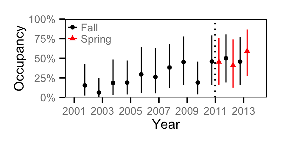
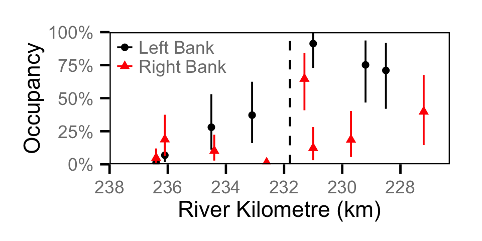
Occupancy - Redside Shiner
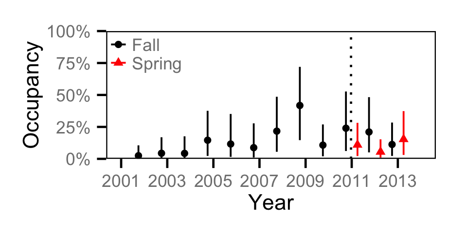
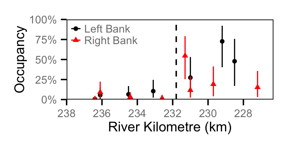
Occupancy - Sculpin
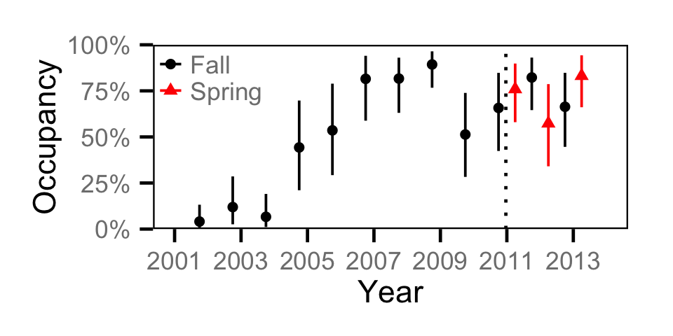
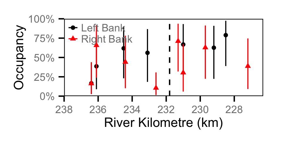
Count - Bull Trout
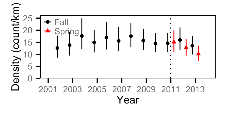
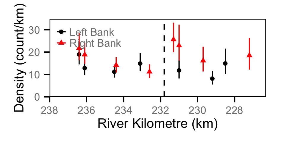
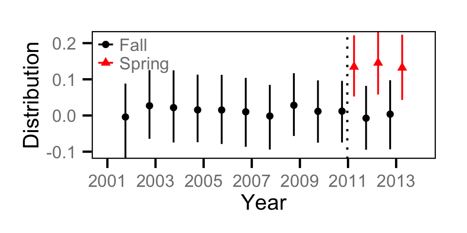
Count - Burbot
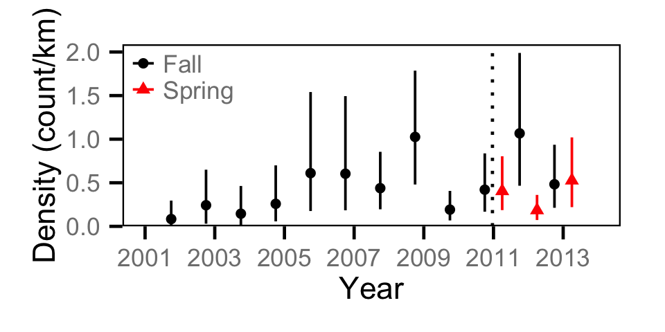
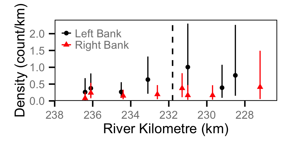
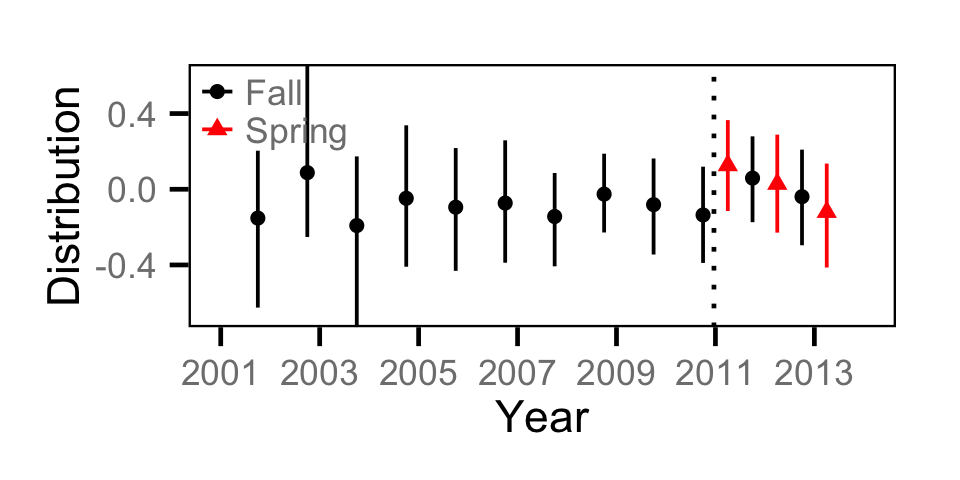
Count - Mountain Whitefish
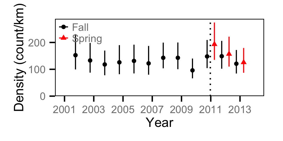
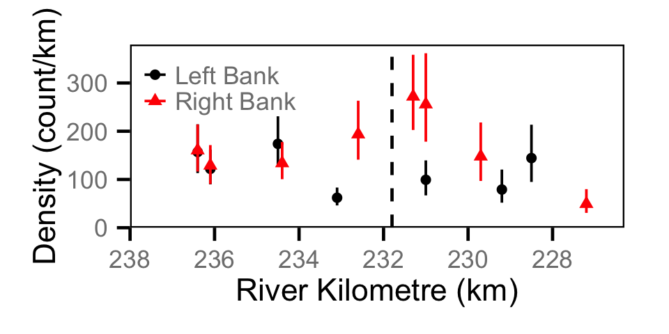
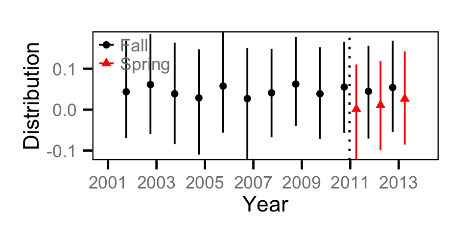
Count - Northern Pikeminnow
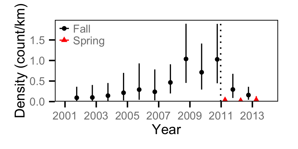
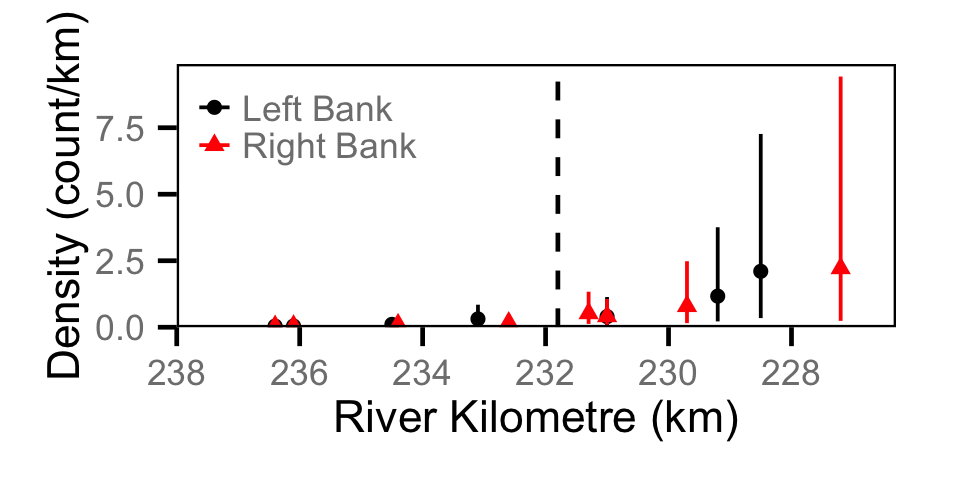
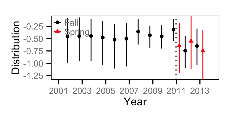
Count - Rainbow Trout
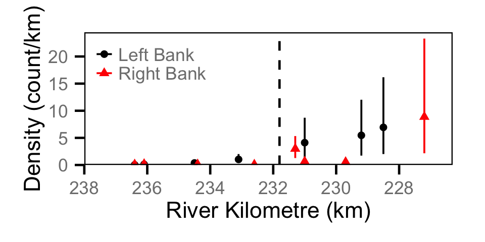
Count - Suckers
Catch - Adult BT
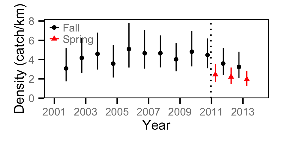
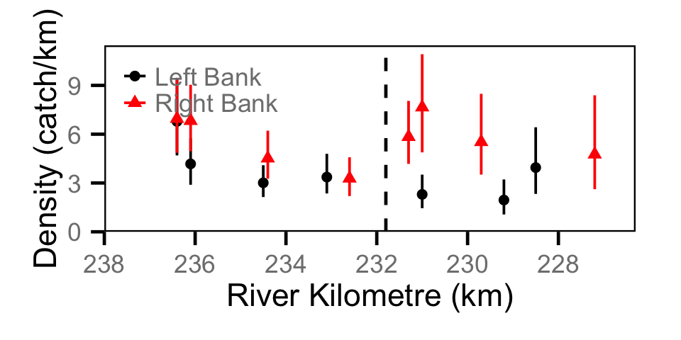
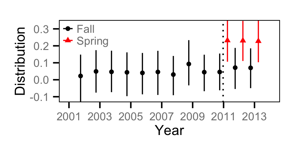
Catch - Adult CSU
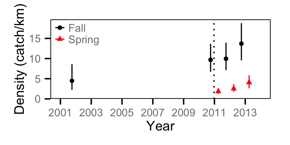
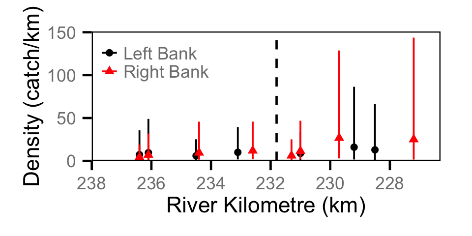
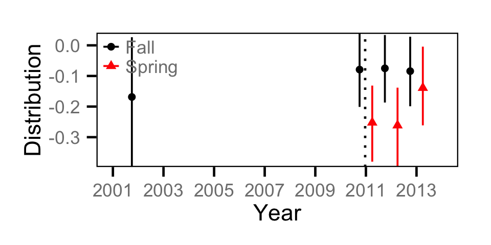
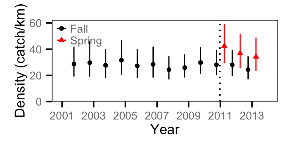
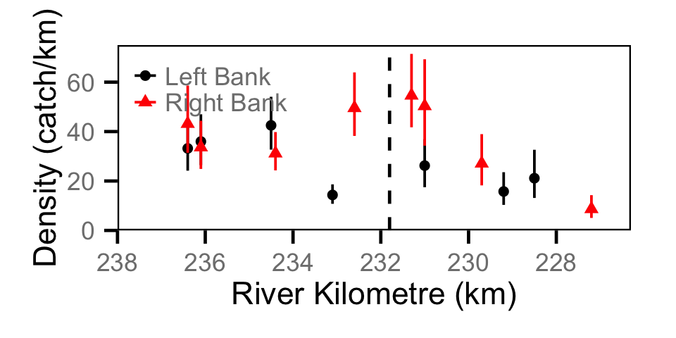
Catch - Adult MW
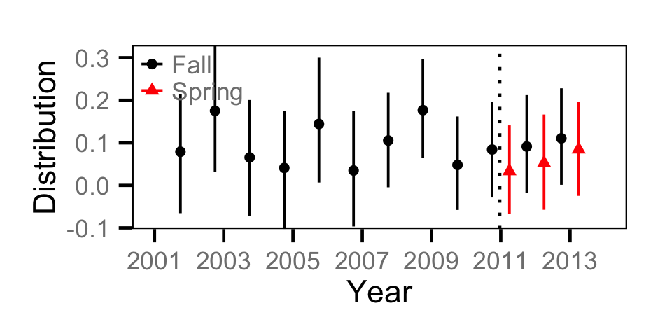
Catch - Adult RB
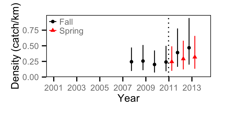
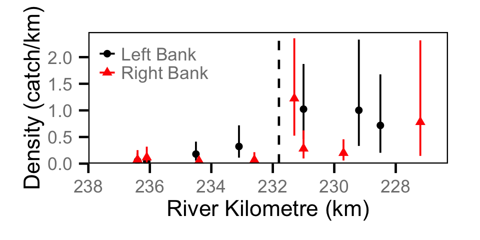
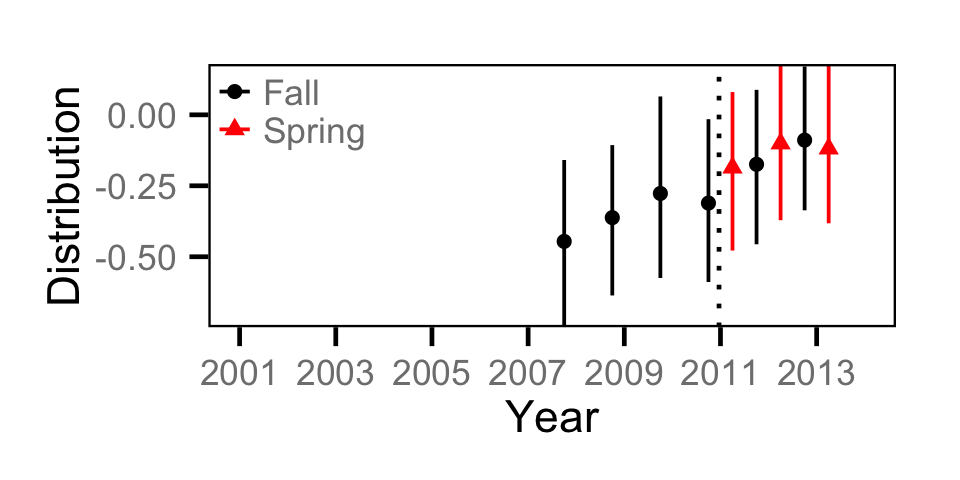
Catch - Juvenile BT
Catch - Juvenile MW
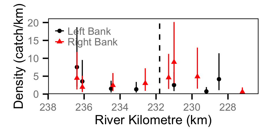
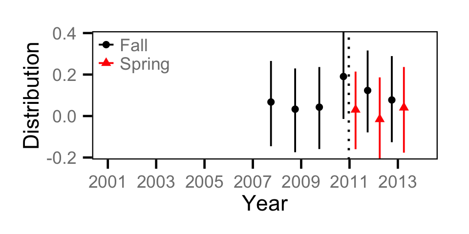
Site Fidelity - Adult BT
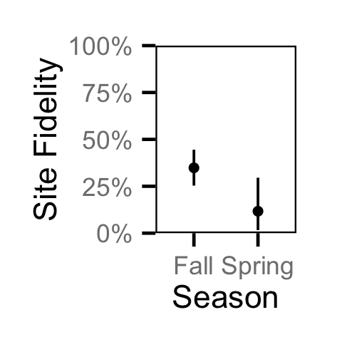
Site Fidelity - Adult CSU
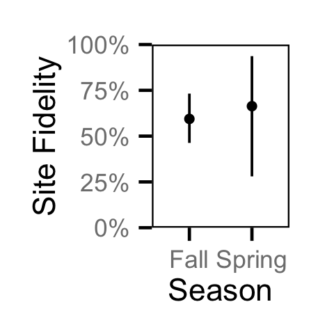
Site Fidelity - Adult MW
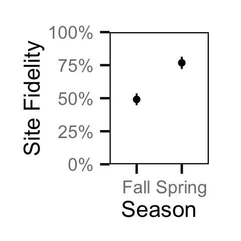
Site Fidelity - Adult RB
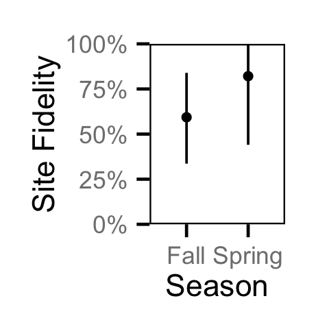
Site Fidelity - Juvenile BT
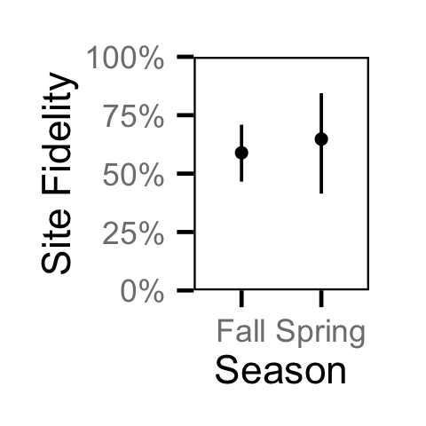
Site Fidelity - Juvenile MW
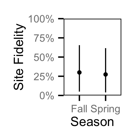
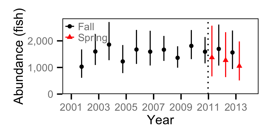
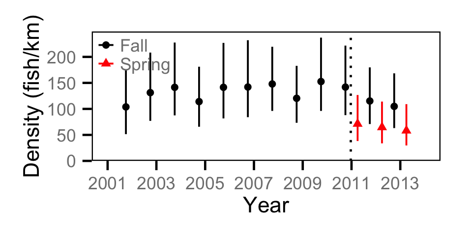
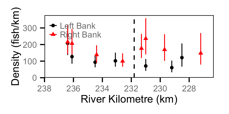
Abundance - Adult BT
Abundance - Adult CSU
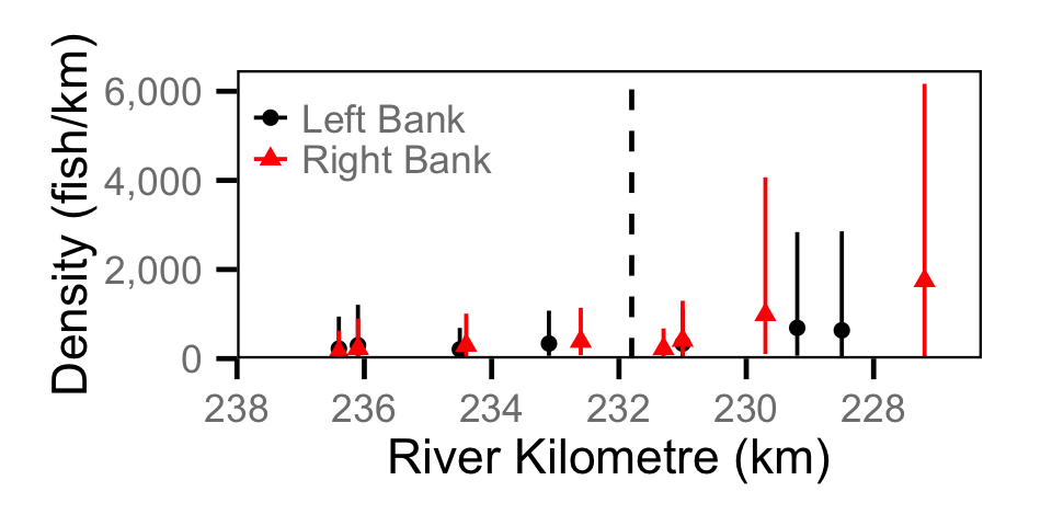
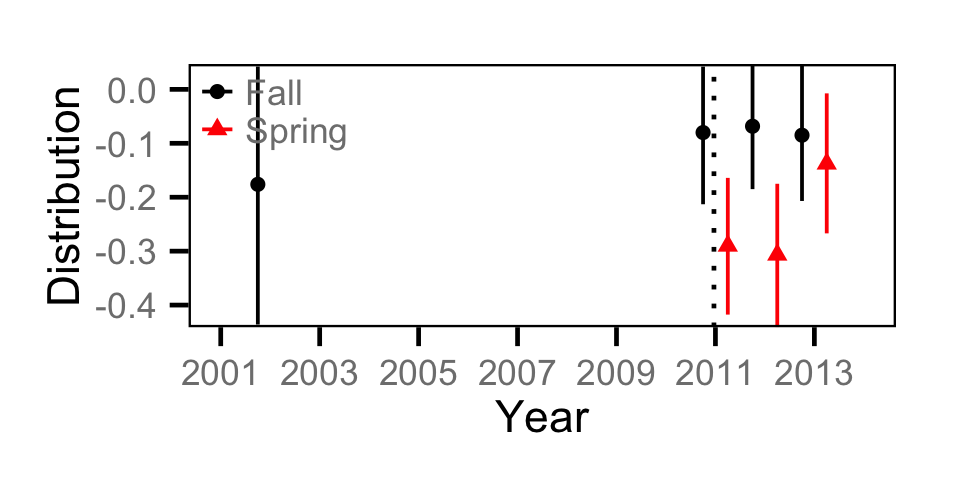
Abundance - Adult MW
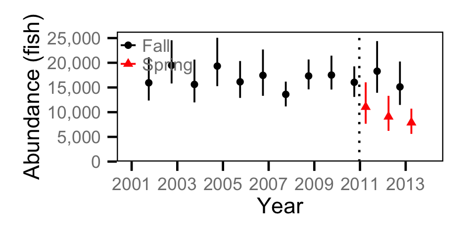
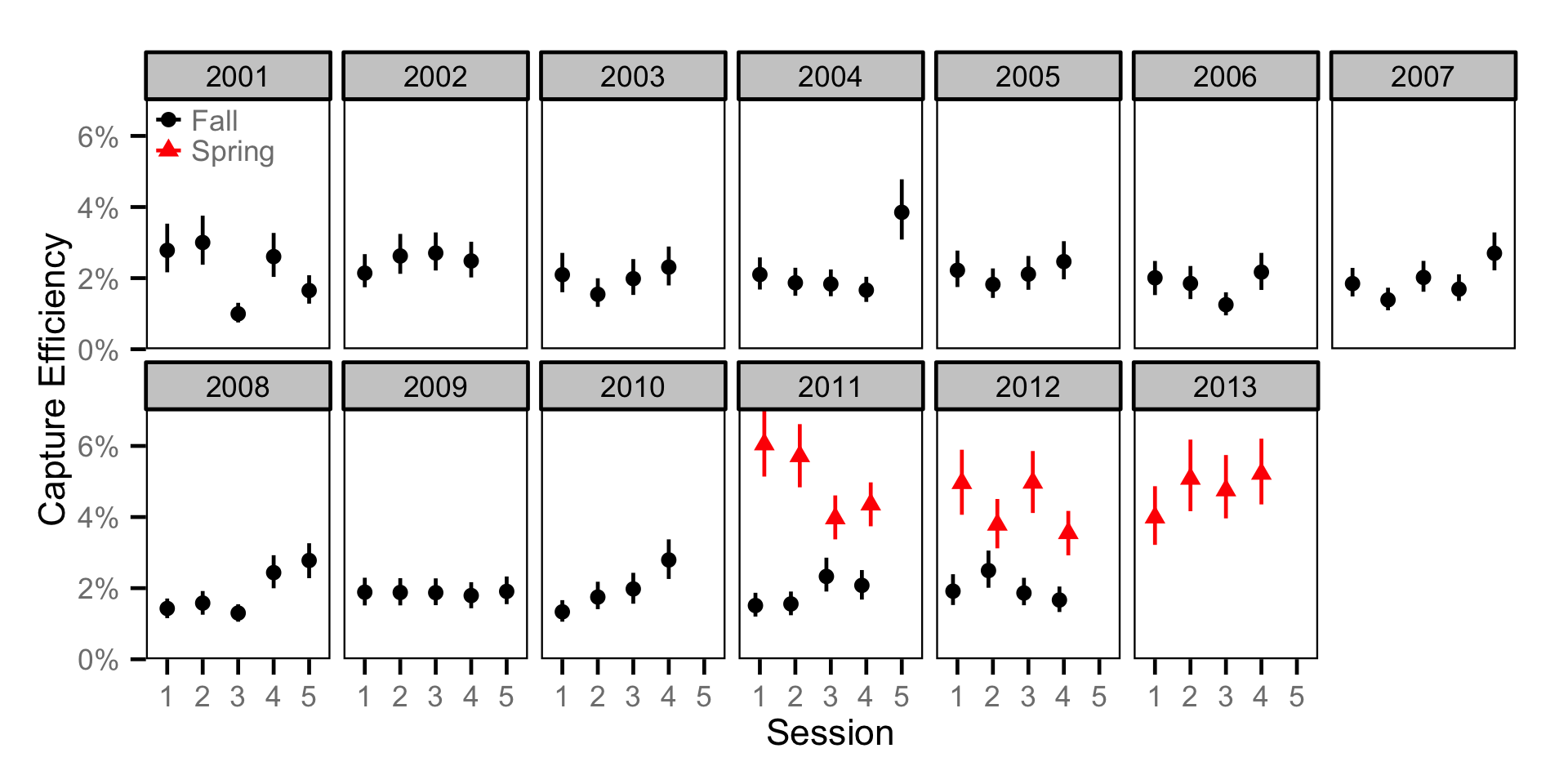
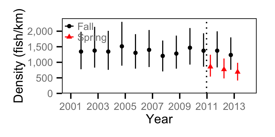
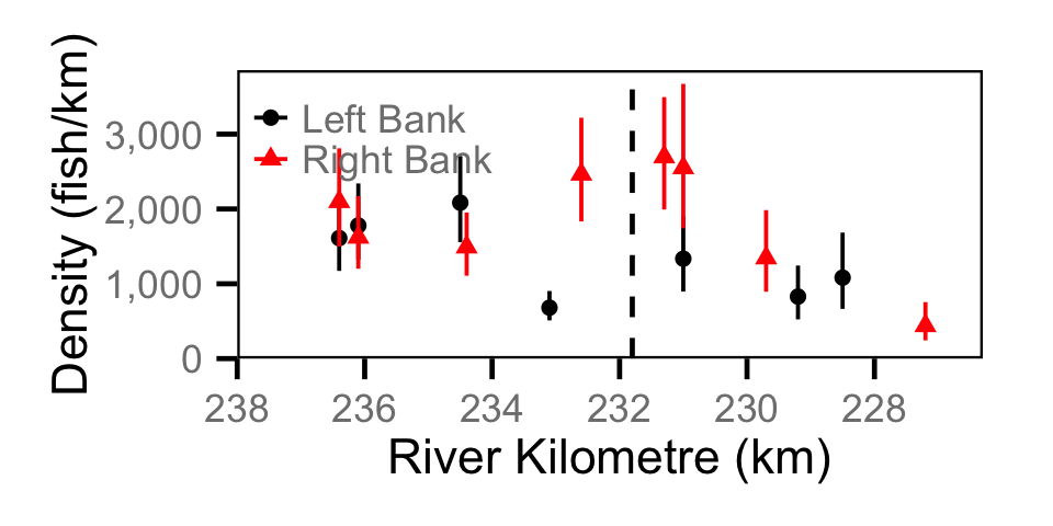
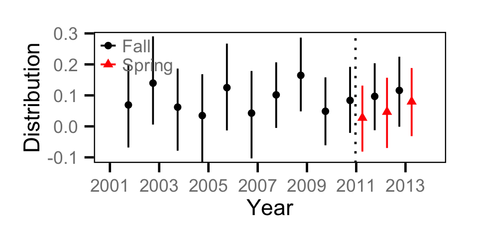
Abundance - Juvenile MW
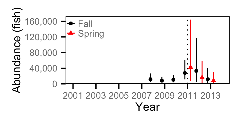
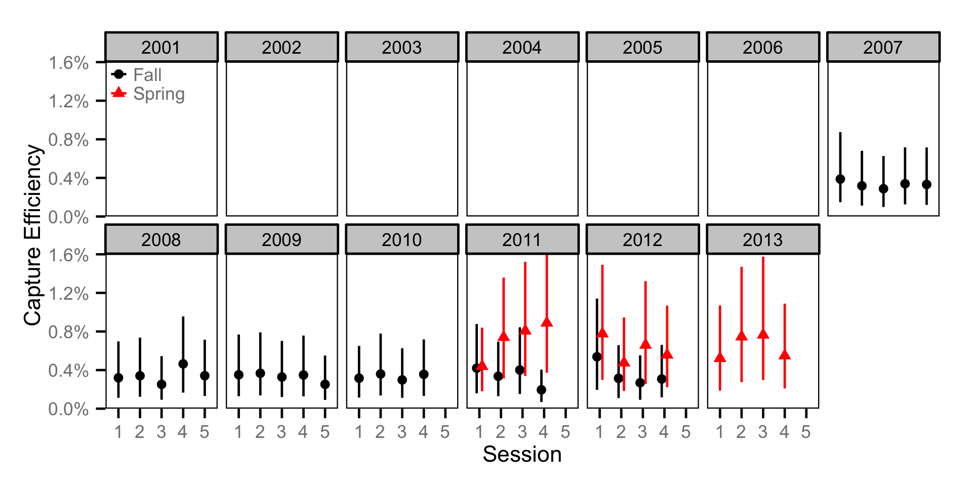
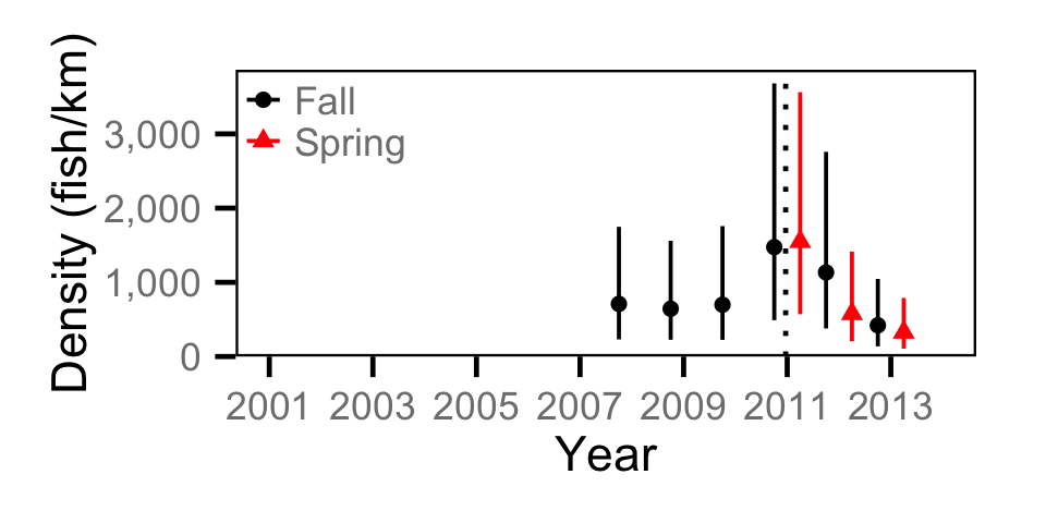
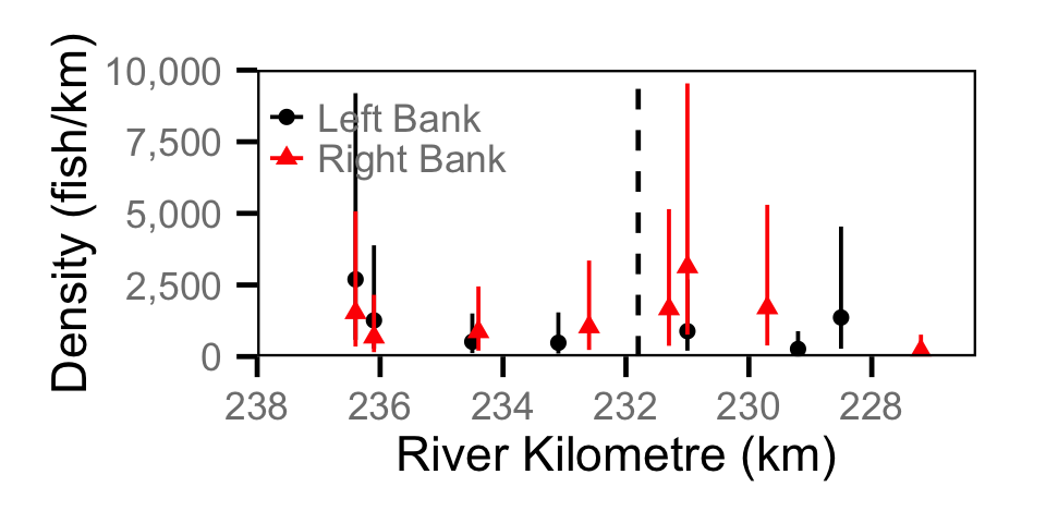

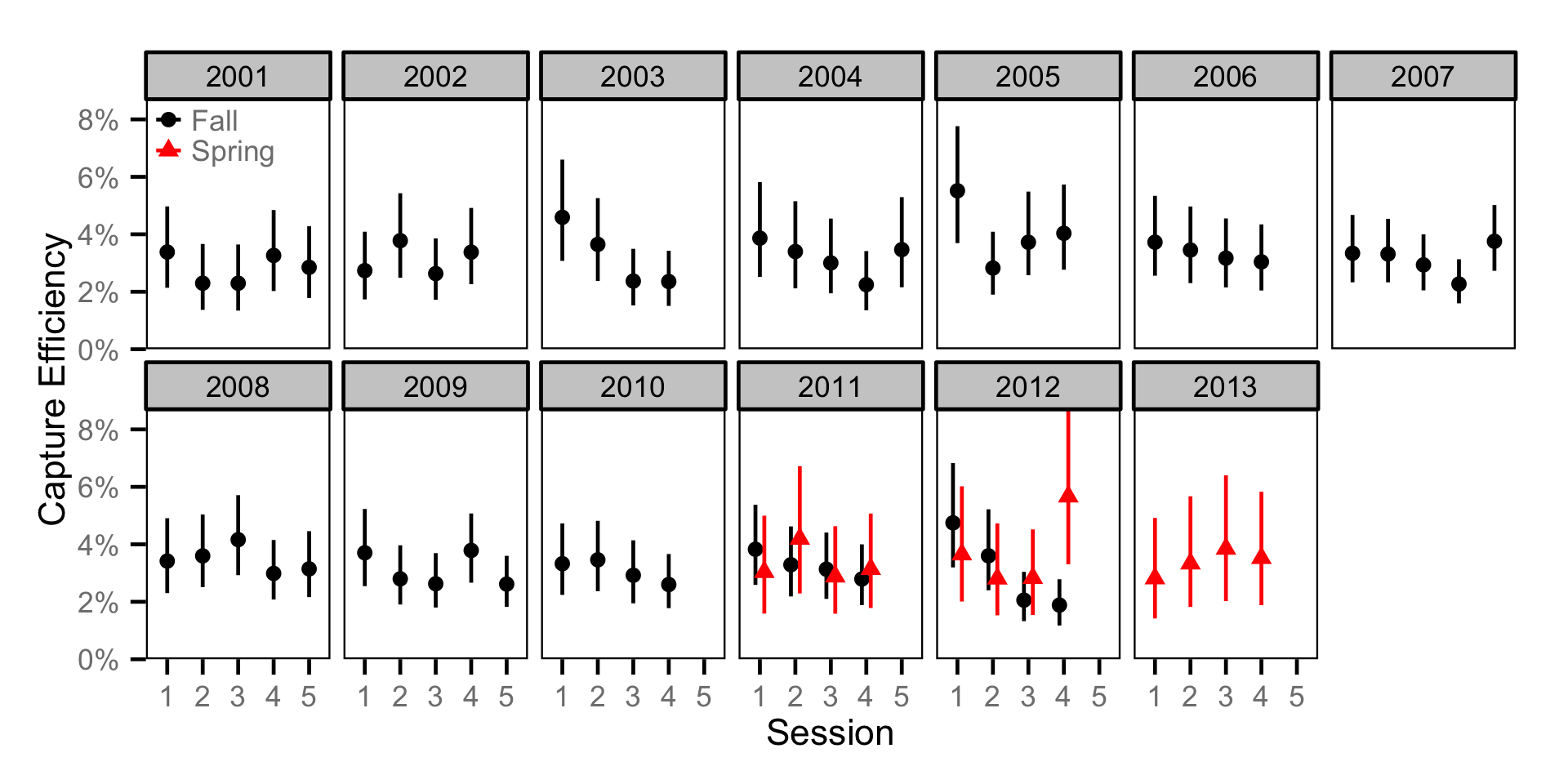
Capture Efficiency - Adult BT
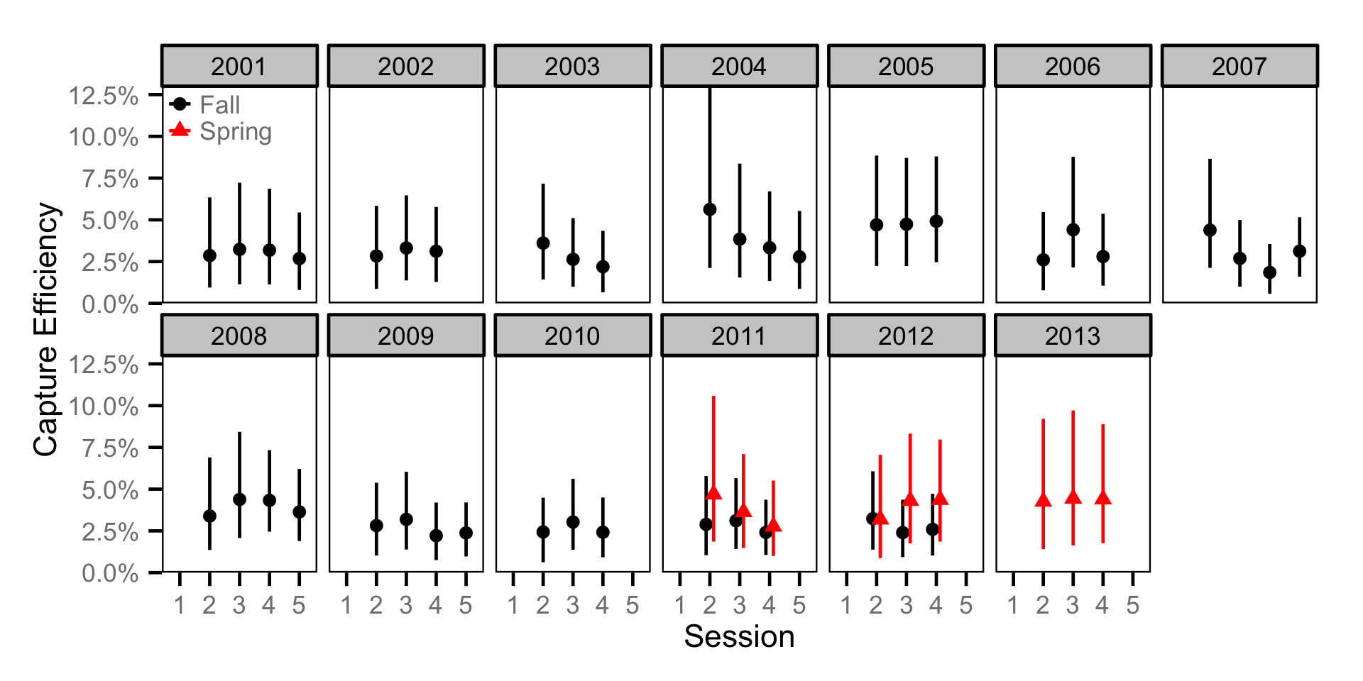
Capture Efficiency - Adult CSU
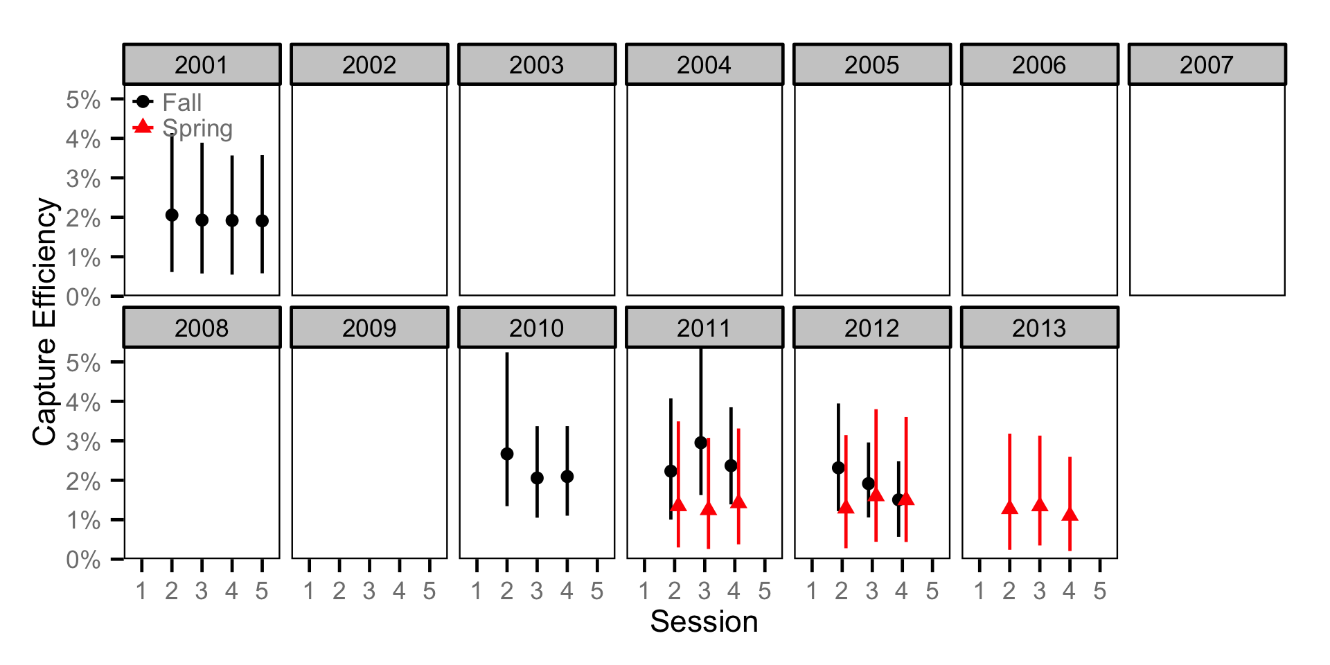
Capture Efficiency - Adult MW
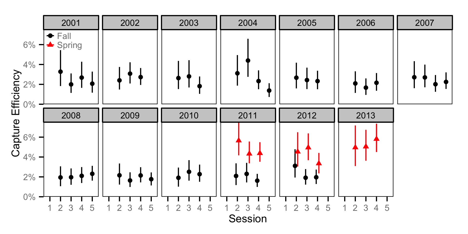
Capture Efficiency - Adult RB
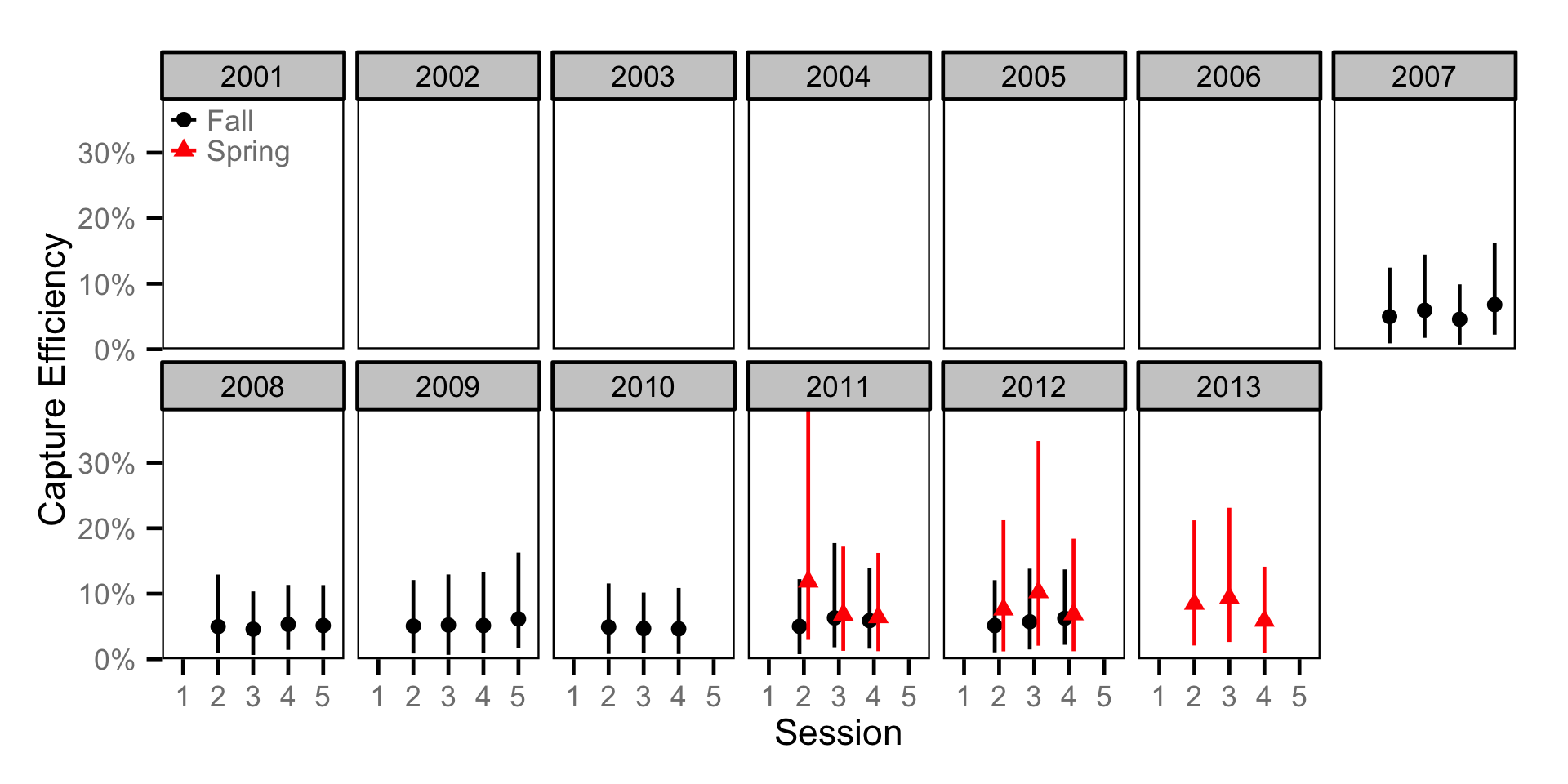
Capture Efficiency - Juvenile BT
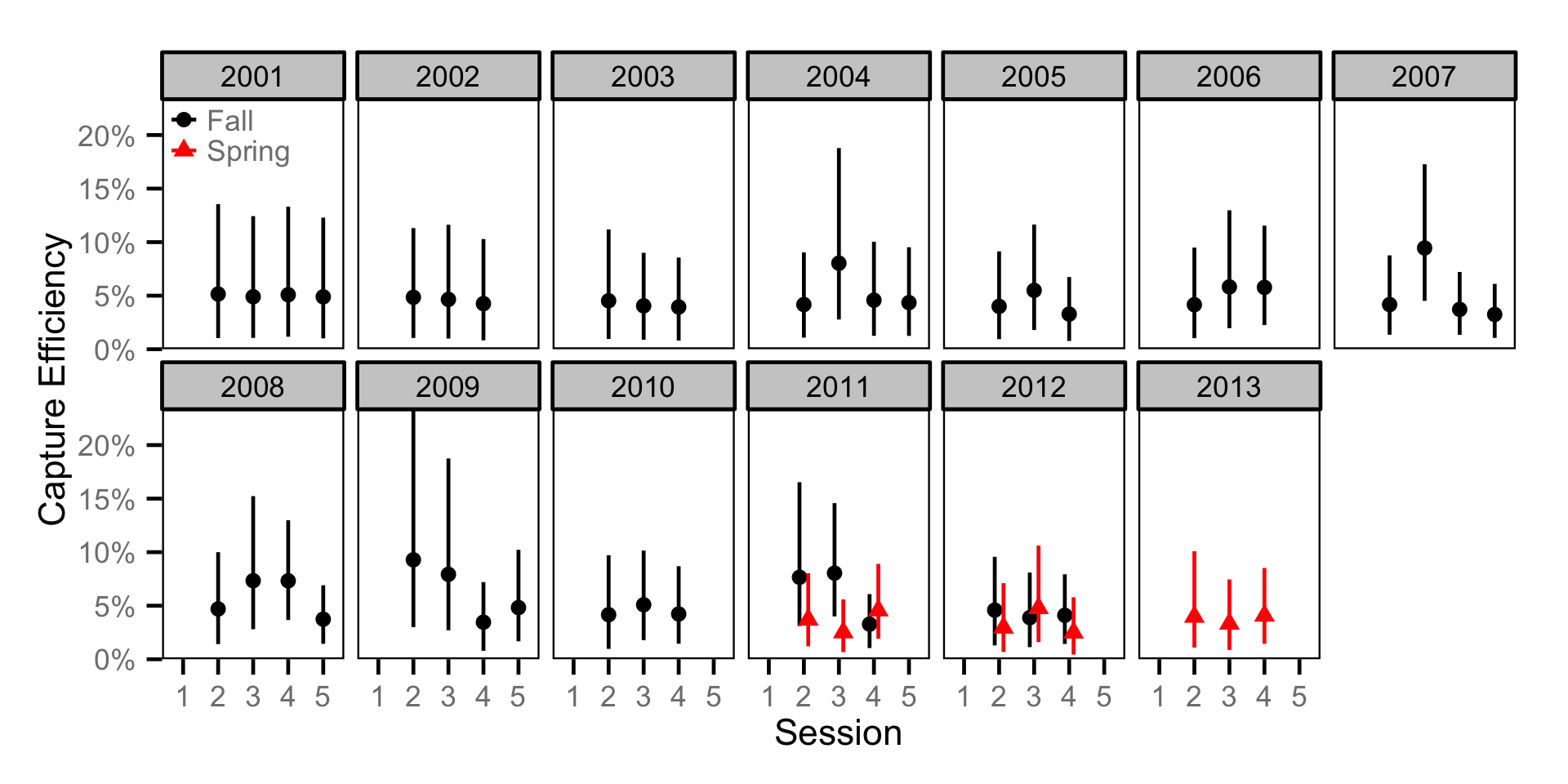
Capture Efficiency - Juvenile MW
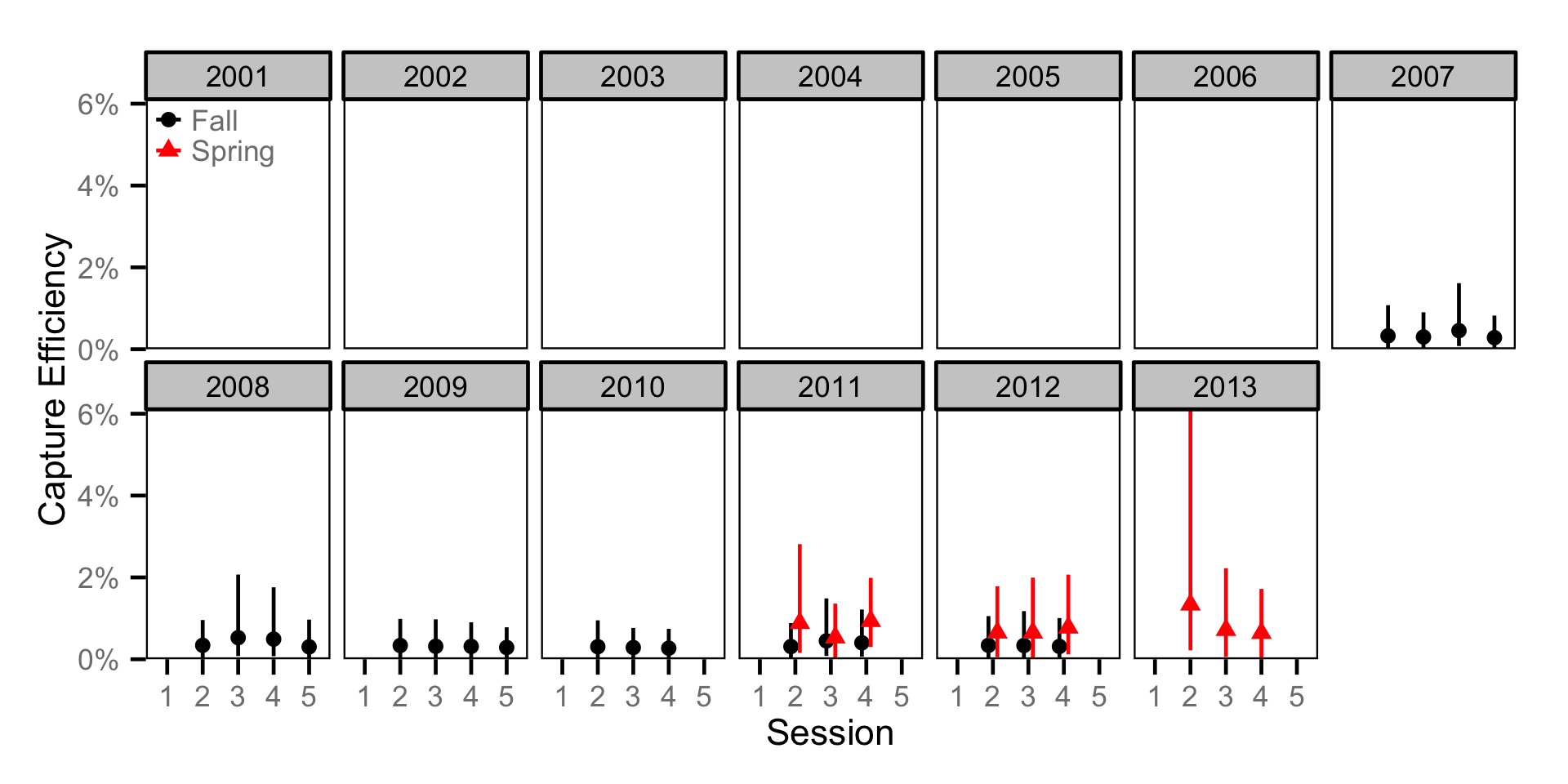
Growth - Bull Trout
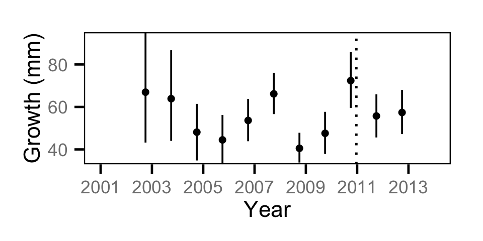
Growth - Mountain Whitefish
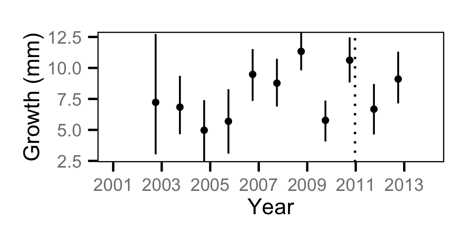
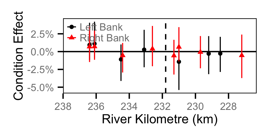
Condition - Adult BT
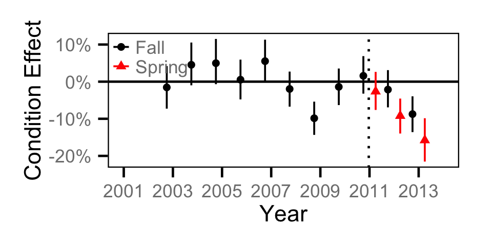
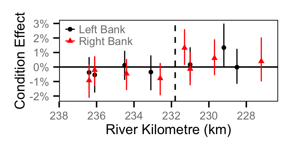
Condition - Adult MW

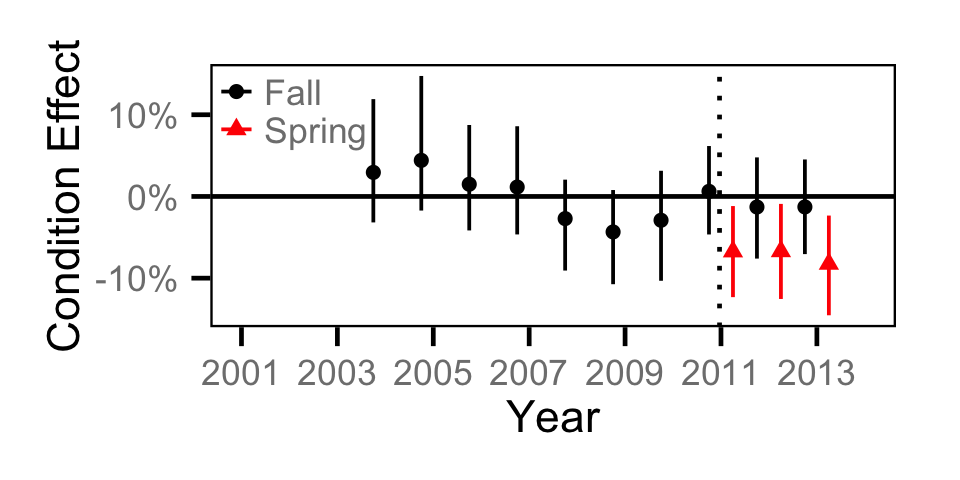
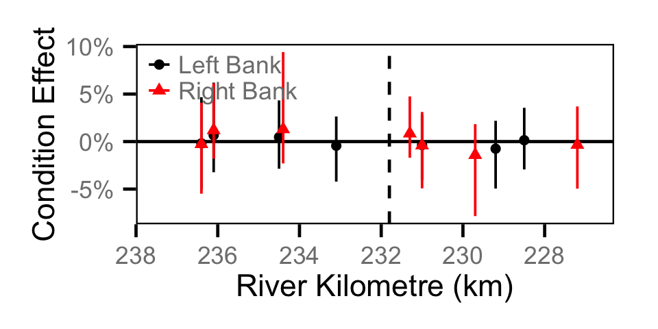
Condition - Adult RB
Condition - Juvenile BT
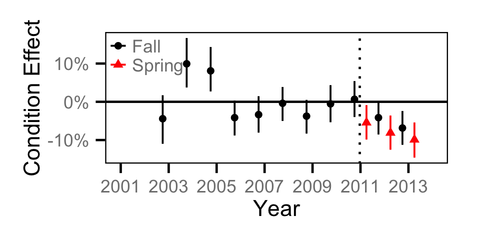
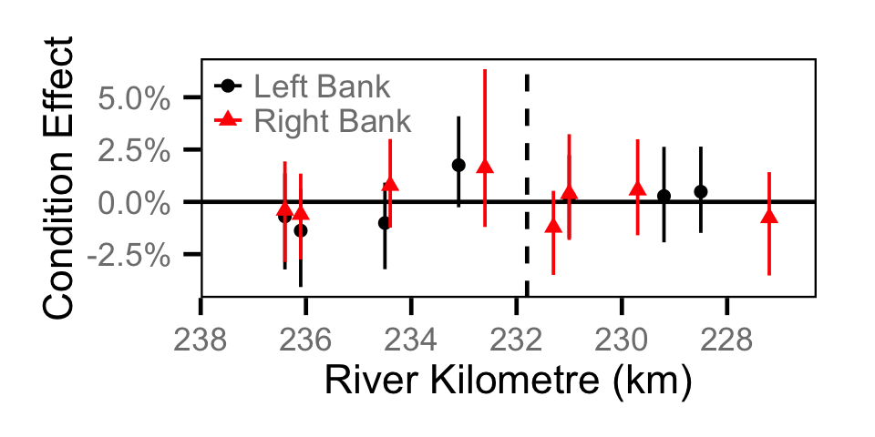
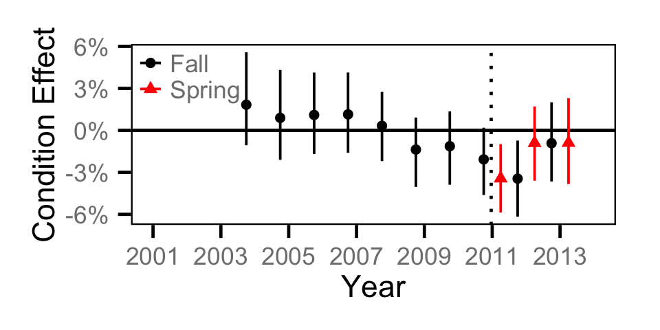
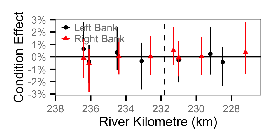
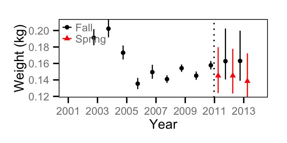
Condition - Juvenile MW
Biomass - Adult BT
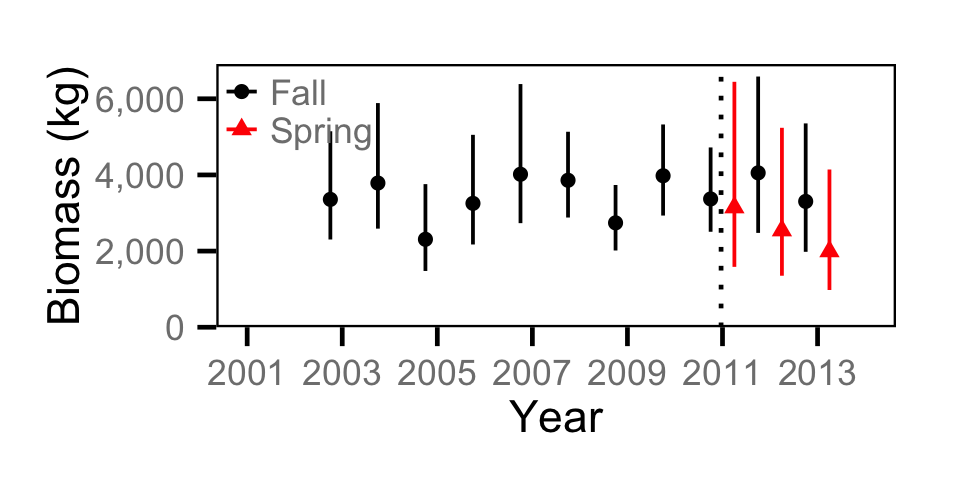
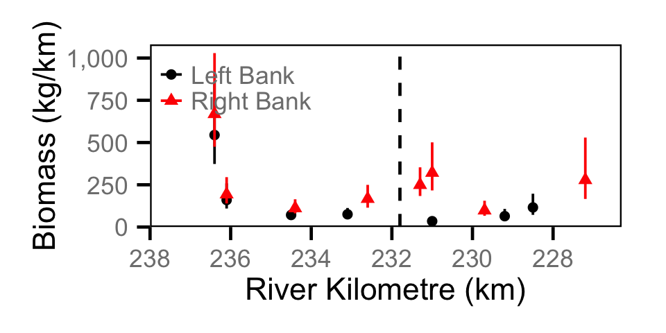
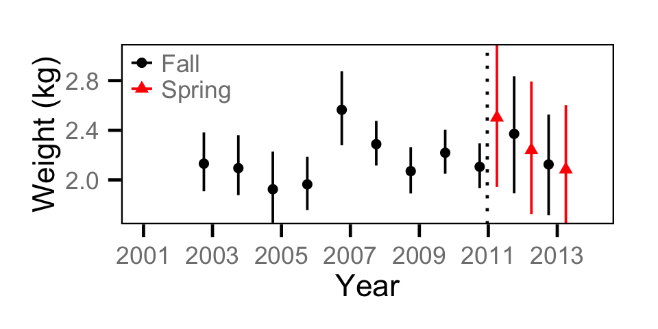
Biomass - Adult MW
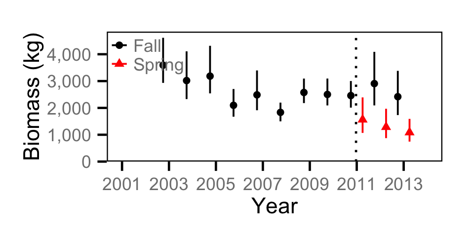
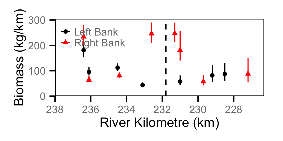
Biomass - Juvenile MW
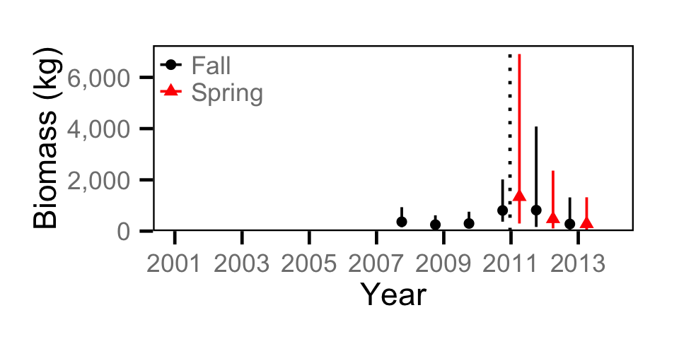
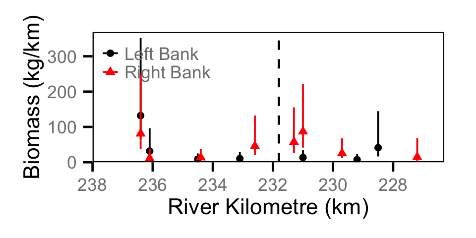
Multivariate Analysis - Eigen Vector
Multivariate Analysis - Environmental
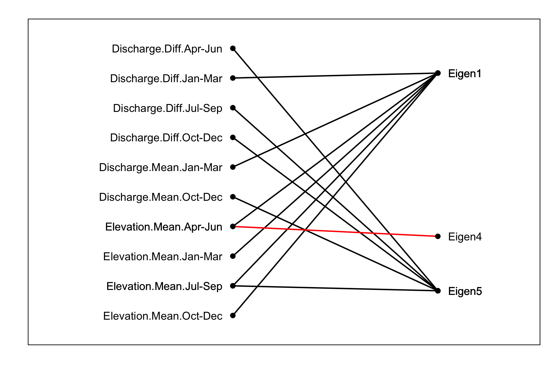
Multivariate Analysis - Indexing
Significance
The following table summarises the significance levels for the management hypotheses tested in the analyses.
| Parameter | Analysis | Species | Stage | Significance | Direction |
|---|---|---|---|---|---|
| Growth | Growth | Bull Trout | All | 0.8802 | |
| Growth | Growth | Mountain Whitefish | All | 0.9507 | |
| Condition | Condition | Bull Trout | Juvenile | 0.1140 | |
| Condition | Condition | Bull Trout | Adult | 0.0444 | - |
| Condition | Condition | Mountain Whitefish | Juvenile | 0.3772 | |
| Condition | Condition | Mountain Whitefish | Adult | 0.0000 | - |
| Condition | Condition | Rainbow Trout | Adult | 0.6647 | |
| Abundance | Count | Bull Trout | All | 0.2914 | |
| Abundance | Abundance | Bull Trout | Adult | 0.3114 | |
| Abundance | Count | Mountain Whitefish | All | 0.7063 | |
| Abundance | Abundance | Mountain Whitefish | Juvenile | 0.4199 | |
| Abundance | Abundance | Mountain Whitefish | Adult | 0.6806 | |
| Abundance | Count | Rainbow Trout | All | 0.0279 | + |
| Abundance | Count | Burbot | All | 0.1058 | |
| Abundance | Count | Northern Pikeminnow | All | 0.6707 | |
| Abundance | Abundance | Sucker (Largescale) | Adult | 0.2282 | |
| Abundance | Count | Sucker | All | 0.0060 | + |
| Distribution | Count | Bull Trout | All | 0.5788 | |
| Distribution | Abundance | Bull Trout | Adult | 0.6707 | |
| Distribution | Count | Mountain Whitefish | All | 0.8373 | |
| Distribution | Abundance | Mountain Whitefish | Juvenile | 0.8279 | |
| Distribution | Abundance | Mountain Whitefish | Adult | 0.5010 | |
| Distribution | Count | Rainbow Trout | All | 0.1018 | |
| Distribution | Count | Burbot | All | 0.8283 | |
| Distribution | Count | Northern Pikeminnow | All | 0.1277 | |
| Distribution | Abundance | Sucker (Largescale) | Adult | 0.5159 | |
| Distribution | Count | Sucker | All | 0.3752 |
References
- Michael Bradford, Josh Korman, Paul Higgins, (2005) Using confidence intervals to estimate the response of salmon populations (Oncorhynchus spp.) to experimental habitat alterations. Canadian Journal of Fisheries and Aquatic Sciences 62 (12) 2716-2726 10.1139/f05-179
- A Fabens, (1965) Properties and fitting of the Von Bertalanffy growth curve. Growth 29 (3) 265-289
- Hadley Wickham, (2009) ggplot2: elegant graphics for data analysis. http://had.co.nz/ggplot2/book
- Ji He, James Bence, James Johnson, David Clapp, Mark Ebener, (2008) Modeling Variation in Mass-Length Relations and Condition Indices of Lake Trout and Chinook Salmon in Lake Huron: A Hierarchical Bayesian Approach. Transactions of the American Fisheries Society 137 (3) 801-817 10.1577/T07-012.1
- Joseph Thorley, (2014) jaggernaut: An R package to facilitate Bayesian analyses using JAGS (Just Another Gibbs Sampler). https://github.com/joethorley/jaggernaut
- Marc Kery, Michael Schaub, (2011) Bayesian population analysis using {WinBUGS} : a hierarchical perspective.
- Marc Kery, (2010) Introduction to {WinBUGS} for Ecologists: A Bayesian approach to regression, {ANOVA}, mixed models and related analyses. http://public.eblib.com/EBLPublic/PublicView.do?ptiID=629953
- M. Plummer, (2012) {JAGS} Version 3.3.0 User Manual. http://sourceforge.net/projects/mcmc-jags/files/Manuals/3.x/
- R Team, (2013) R: A Language and Environment for Statistical Computing. http://www.R-project.org
- L. Bertalanffy, (1938) A quantitative theory of organic growth (inquiries on growth laws ii). Human Biology 10 181-213
Acknowledgements
The organisations and individuals whose contributions have made this analysis report possible include:
- BC Hydro
- Guy Martel
- Karen Bray
- Jason Watson
- Okanagan National Alliance
- Charlotte Whitney
- Michael Zimmer
- Golder Associates
- Dustin Ford
- David Roscoe
- Sima Usvyatsov
- Dana Schmidt
- Larry Hildebrand