Quesnel Lake Exploitation Analysis 2018
The suggested citation for this analytic report is:
Dalgarno, S. and Thorley, J.L. (2019) Quesnel Lake Exploitation Analysis 2018. A Poisson Consulting Analysis Report. URL: https://www.poissonconsulting.ca/f/1356175666.
Background
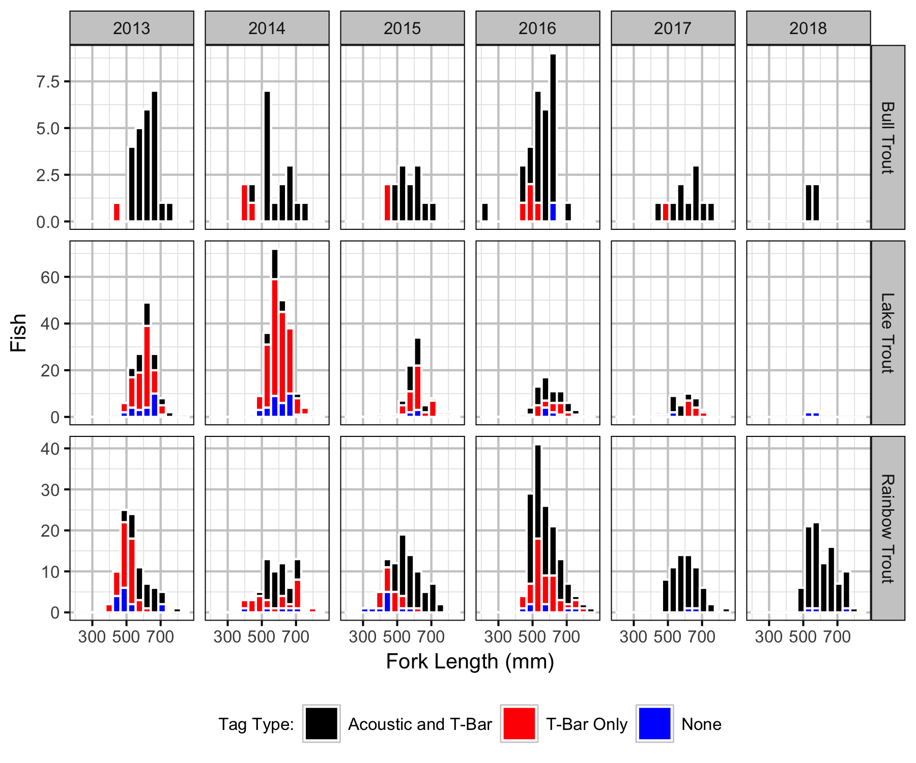
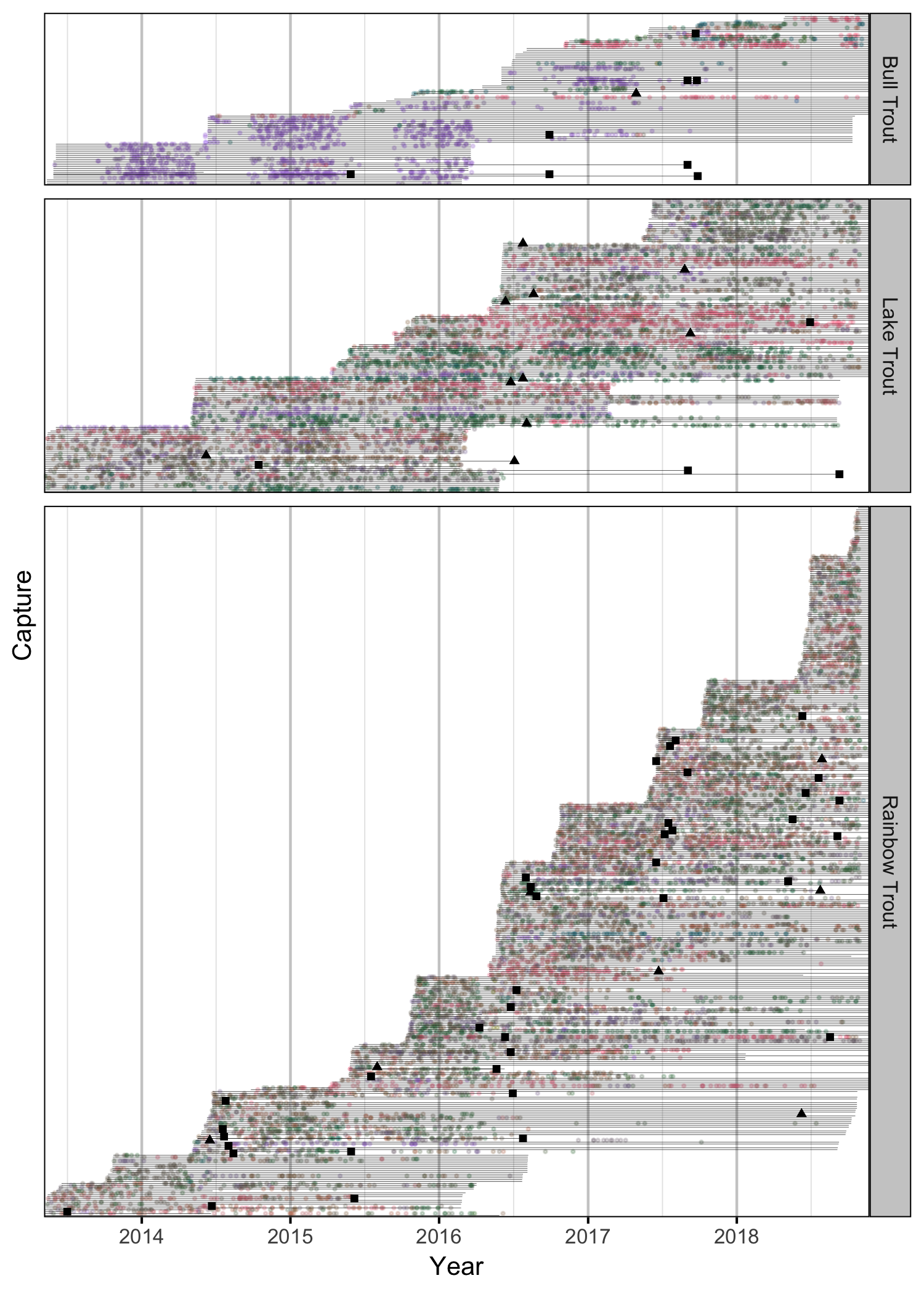
Quesnel Lake supports a recreational fishery for large Bull Trout, Lake Trout and Rainbow Trout. To provide information on the natural and fishing mortality, trout were caught by angling and tagged with acoustic transmitters and/or reward tags.
Methods
Data Preparation
The outing, receiver deployment, detection, fish capture and recapture information were provided by the Ministry of Forests, Lands and Natural Resource Operations and added to a SQLite database.
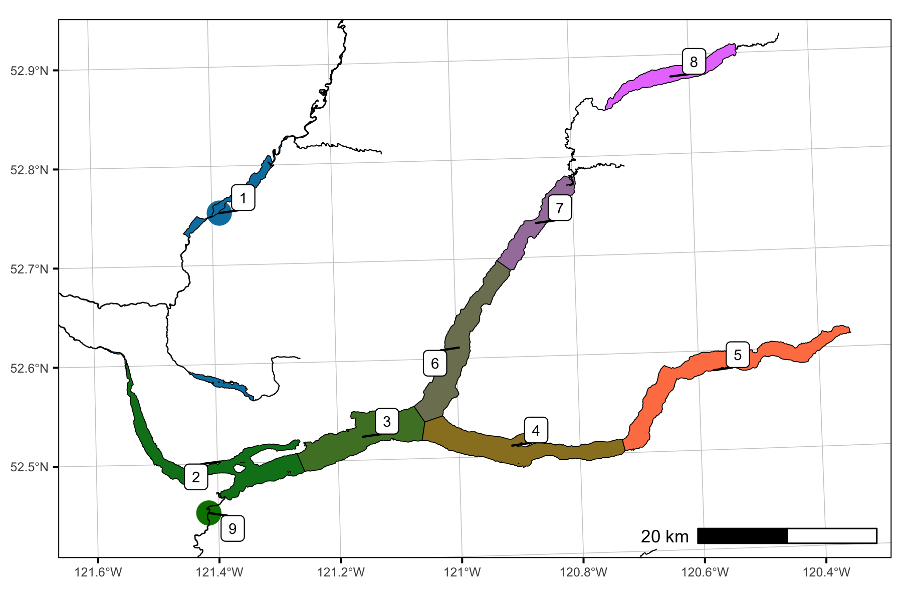
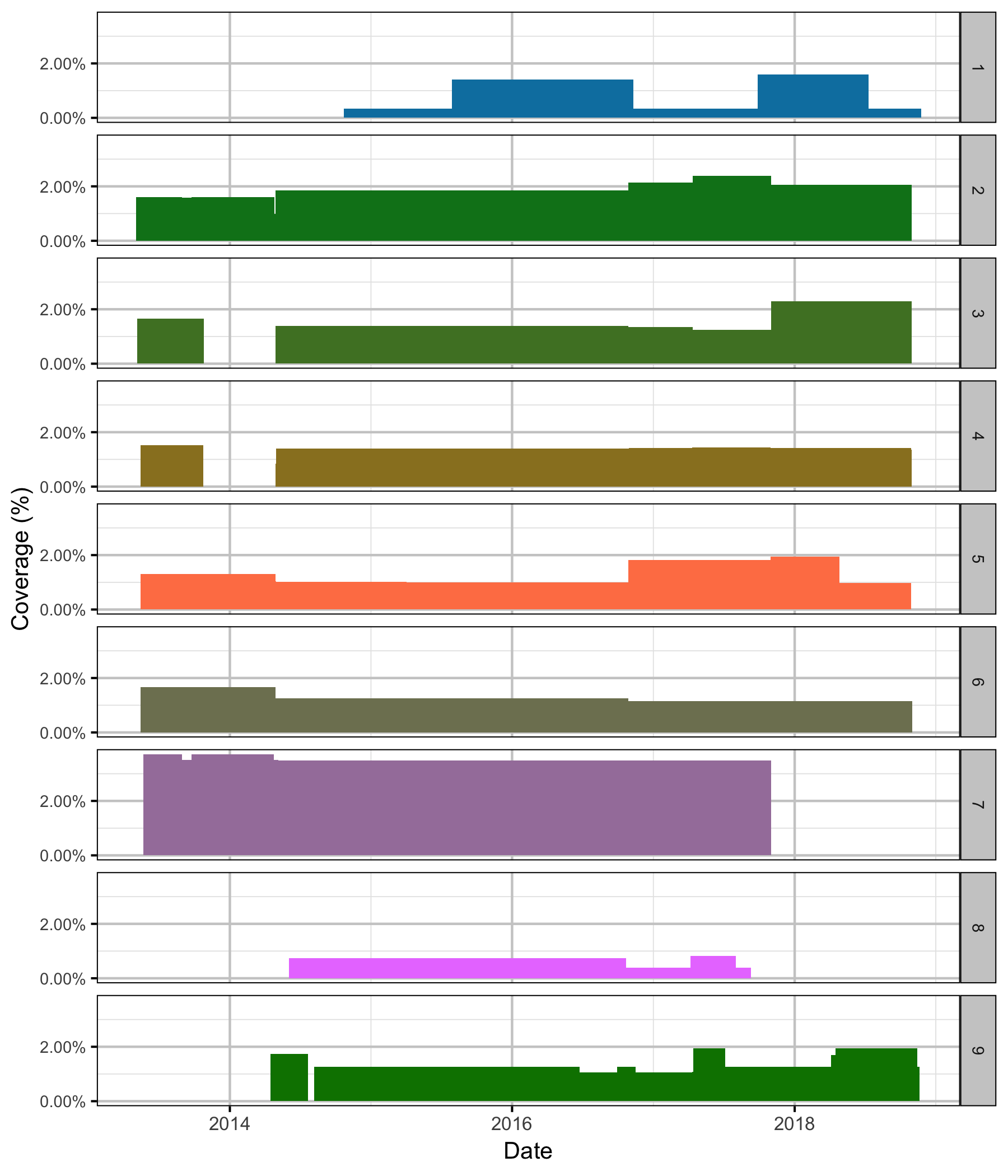
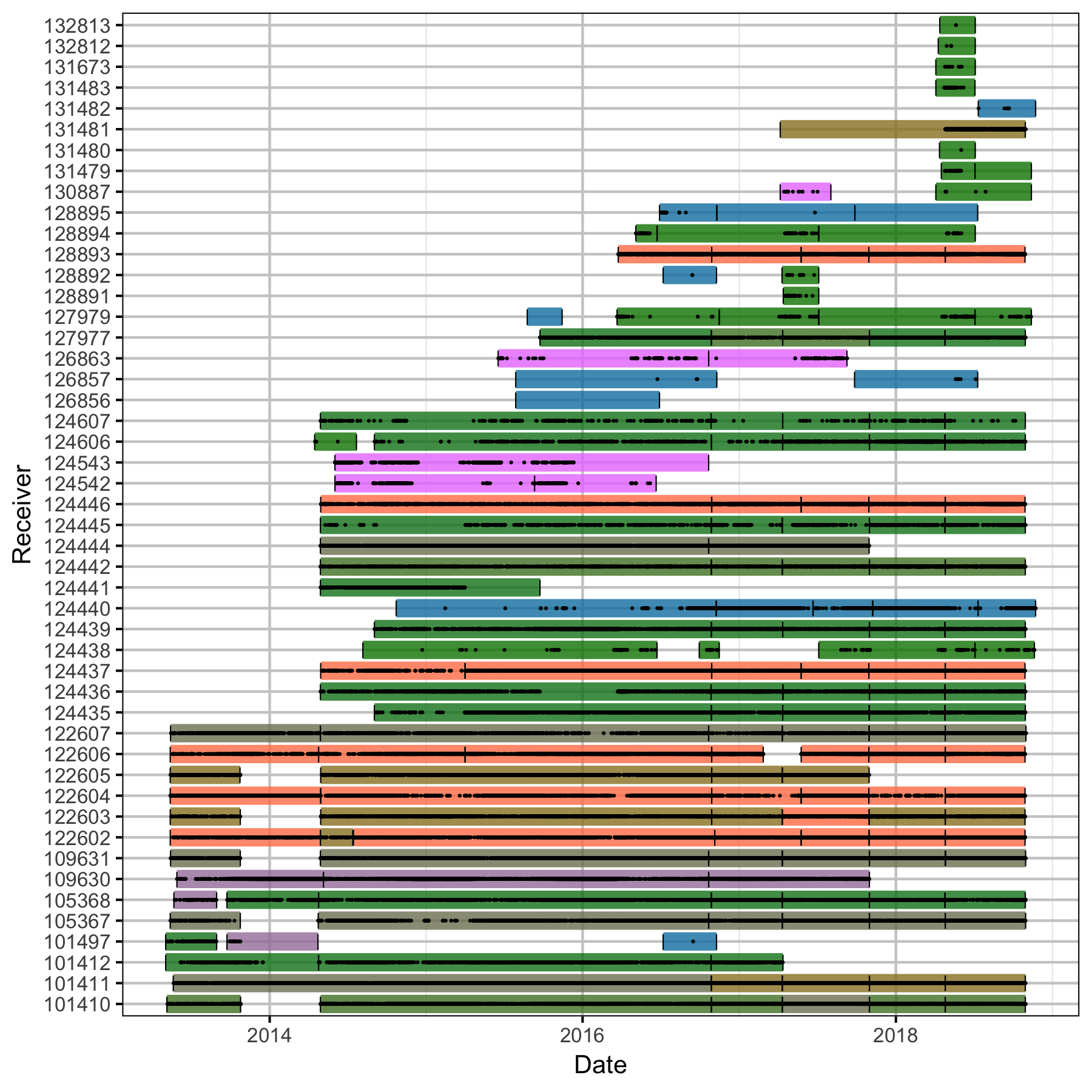
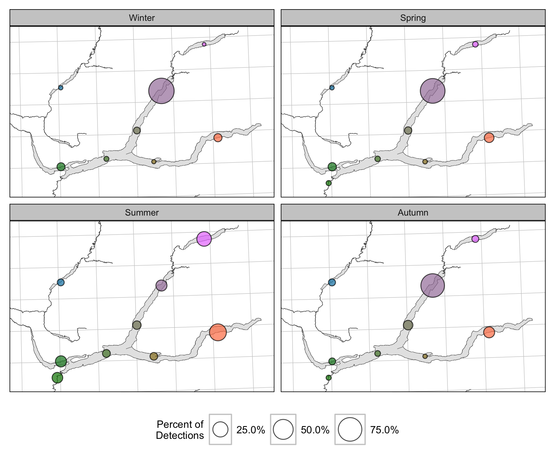
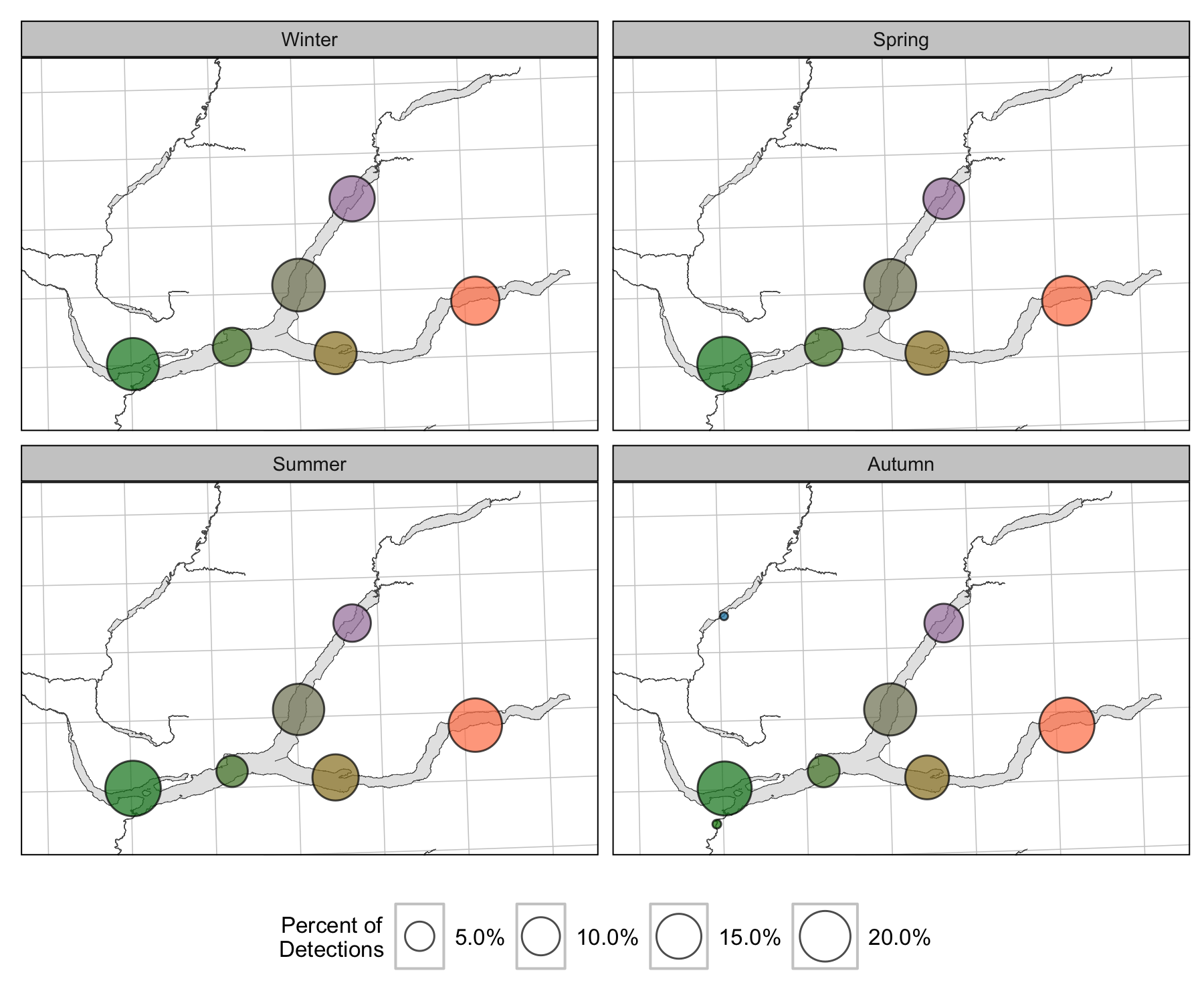
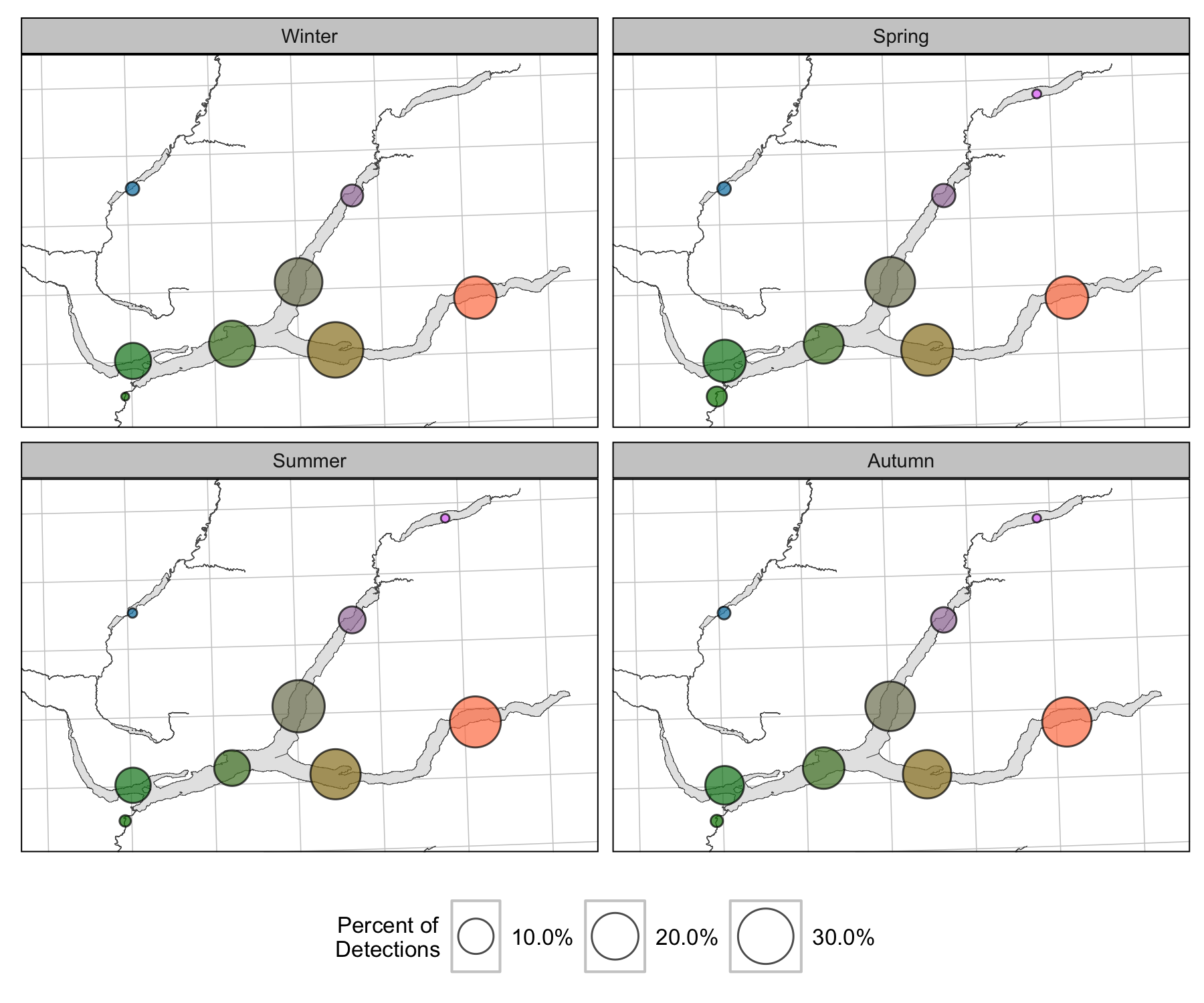
The data were prepared for analysis using R version 3.5.3 (R Core Team 2018). Receivers were assumed to have a detection range of 500 m. Detections were aggregated daily, where for each transmitter the receiver with the most number of detections was chosen. In the case of a tie, the receiver with the greatest coverage area was chosen. Only individuals with a fork length (FL) \(\geq\) 450 mm, an acoustic tag life \(\geq\) 365 days (if acoustically tagged) and a $100 and $10 reward tags were included in the survival analysis.
The Seasons were Winter (December - February), Spring (March - May), Summer (June - August) and Autumn (September - November).
Data Analysis
Hierarchical Bayesian models were fitted to the data using R version
3.5.3 (R Core Team 2018) and JAGS 4.2.0 (Plummer 2015) which
interfaced with each other via the jmbr package. For additional
information on hierarchical Bayesian modelling in the BUGS language, of
which JAGS uses a dialect, the reader is referred to Kery and Schaub (2011, 41–44).
Unless indicated otherwise, the Bayesian analyses used normal and uniform prior distributions that were vague in the sense that they did not constrain the posteriors (Kery and Schaub 2011, 36). The posterior distributions were estimated from 1500 Markov Chain Monte Carlo (MCMC) samples thinned from the second halves of 3 chains (Kery and Schaub 2011, 38–40). Model convergence was confirmed by ensuring that \(\hat{R} \leq 1.05\) (Kery and Schaub 2011, 40) and \(\textrm{ESS} \geq 150\) for each of the monitored parameters (Kery and Schaub 2011, 61). Where \(\hat{R}\) is the potential scale reduction factor and \(\textrm{ESS}\) is the effective sample size (Brooks et al. 2011).
The posterior distributions of the fixed (Kery and Schaub 2011, 75) parameters are summarised in terms of the point estimate, standard deviation (sd), the z-score, lower and upper 95% confidence/credible limits (CLs) and the p-value (Kery and Schaub 2011, 37, 42). The estimate is the median (50th percentile) of the MCMC samples, the z-score is \(\mathrm{mean}/\mathrm{sd}\) and the 95% CLs are the 2.5th and 97.5th percentiles. A p-value of 0.05 indicates that the lower or upper 95% CL is 0.
The results are displayed graphically by plotting the modeled relationships between particular variables and the response with the remaining variables held constant. In general, continuous and discrete fixed variables are held constant at their mean and first level values respectively while random variables are held constant at their typical values (expected values of the underlying hyperdistributions) (Kery and Schaub 2011, 77–82). Where informative the influence of particular variables is expressed in terms of the effect size (i.e., percent change in the response variable) with 95% CIs (Bradford, Korman, and Higgins 2005). ### Model Descriptions
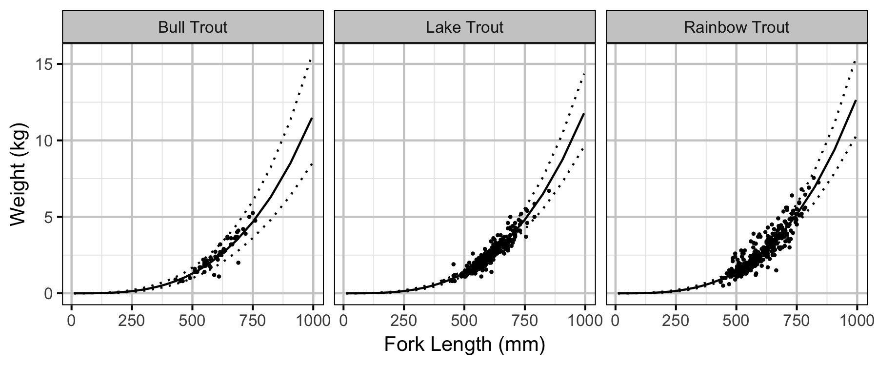
Condition
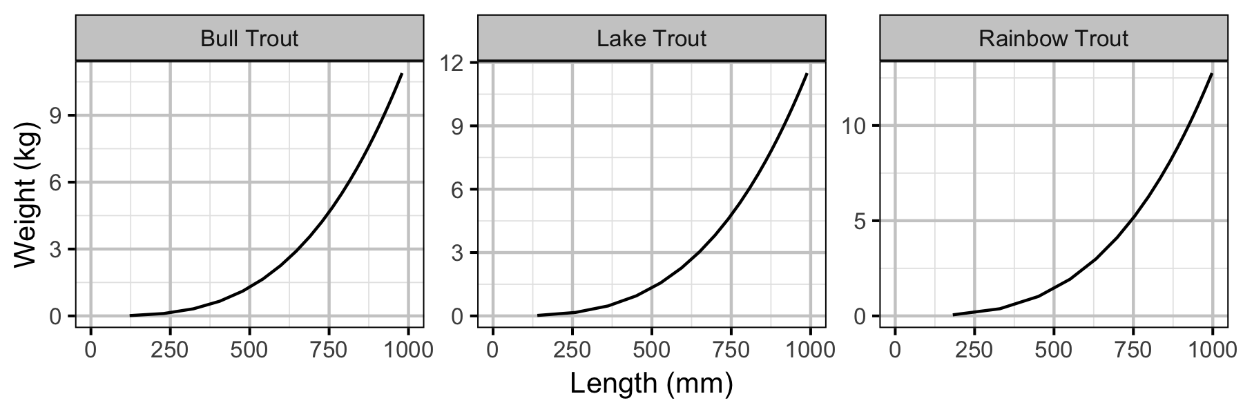
The expected weight of fish of a given length were estimated from the data using a mass-length model (He et al. 2008). Key assumptions of the condition model include:
- The expected weight is allowed to vary with length and date.
- The residual variation in weight is log-normally distributed.
Tag Loss
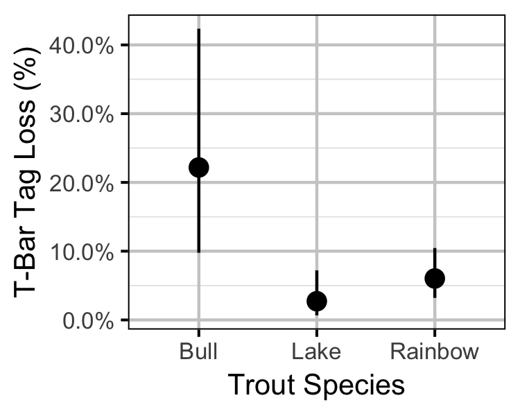
T-bar tag loss was estimated from the number of tags reported from recaught double-tagged individuals (Fabrizio et al. 1999).
Key assumptions of the tag loss model include:
- The probability of tag loss is independent between tags on a fish.
- Reported tag numbers are described by a zero-truncated binomial distribution (as fish that had lost both tags were not reportable).
Survival
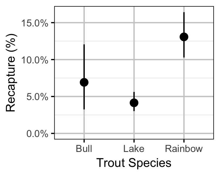
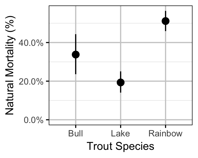
The natural mortality and exploitation were estimated using a Bayesian individual state-space survival model (Thorley and Andrusak 2017) with monthly intervals. The survival model incorporated natural and handling mortality, acoustic detection, inter-section movement, T-bar tag loss, recapture and reporting. In addition to assumptions 1 to 10, in Thorley and Andrusak (2017), the model also assumes that:
- The effect of handling on mortality lasts up to two months after capture.
- Annual T-bar tag-loss is as estimated by the tag loss model.
- All recaptured fish are retained.
- Reporting of recaptured fish with one or more T-bar tags is between 90 and 100%.
Yield-Per-Recruit
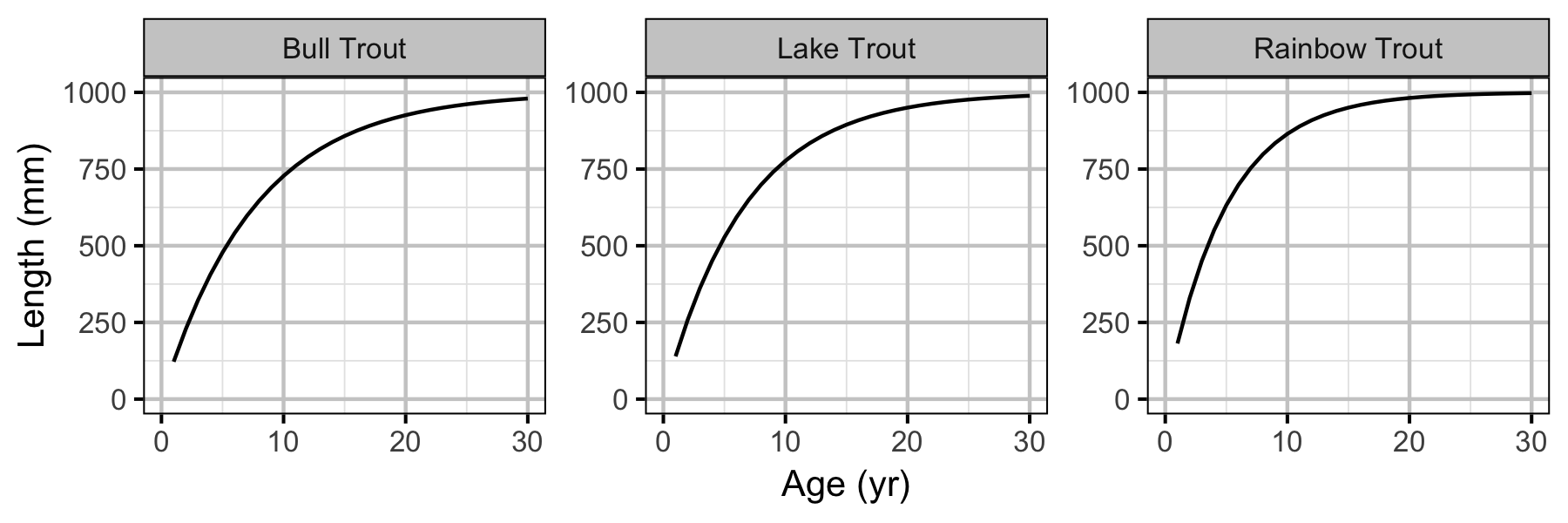
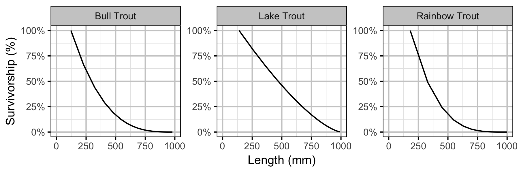
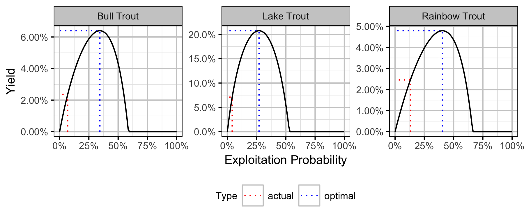
The optimal fishing mortality (to maximize number of individuals harvested) was calculated using a yield-per-recruit approach (Bison, O’Brien, and Martell 2003). Key assumptions include:
- The population is at equilibrium.
- All captured individuals are retained.
- There are no Allee effects.
- There are no limitations on prey species.
- The life-history parameters are fixed.
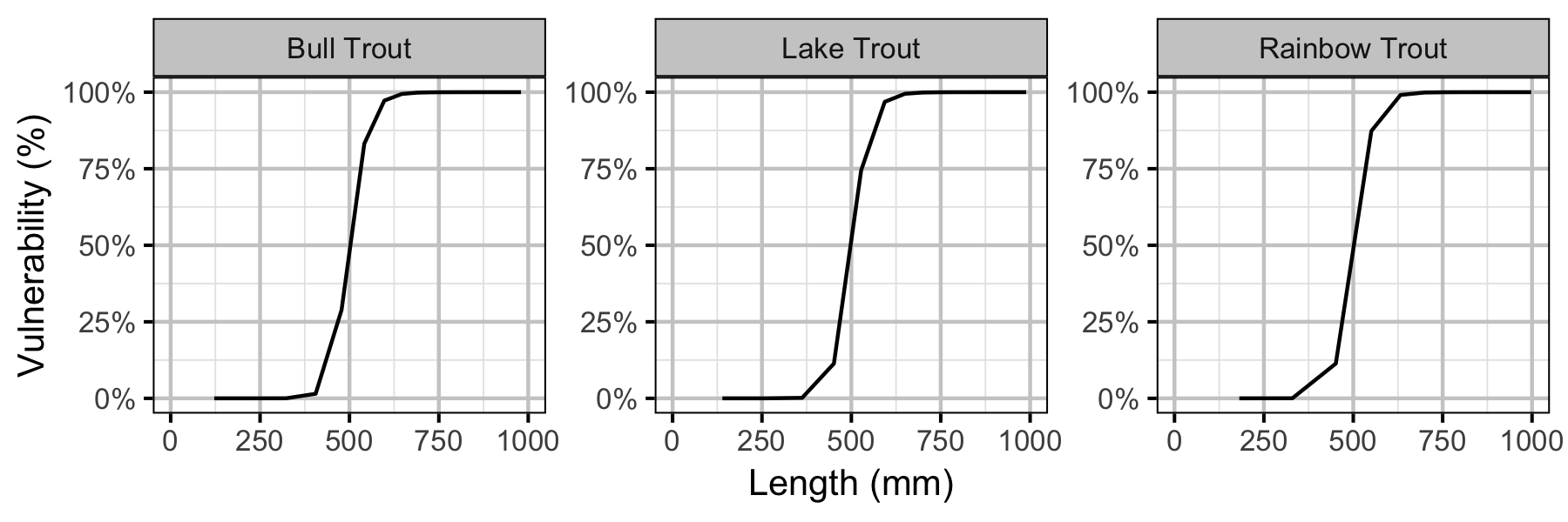
The values of the vulnerability of capture parameters assume that all fish captured during the study are recorded irrespective of length.
Results
Templates
Condition
.model {
               bWeight ~ dnorm(0, 1^-2)
               bWeightLength ~ dnorm(3.18, 0.19^-2)

               sWeight ~ dnorm(0, 1^-2) T(0,)
               for(i in 1:length(LogLength)) {
               eWeight[i] <- bWeight + bWeightLength * LogLength[i]
               Weight[i] ~ dlnorm(eWeight[i], exp(sWeight)^-2)
               }
               }
Block 1. Condition model description.
Tag Loss
model {
  bTagLoss ~ dunif(0,1)
  for (i in 1:nObs) {
    TagsRecap[i] ~ dbin(1 - bTagLoss, 2) T(1, )
  }
..
Block 2. Model description.
Survival
.model{
  bMortality ~ dnorm(-3, 3^-2)
  bMortalityHandling ~ dnorm(0, 2^-2)
  bDetected ~ dunif(0, 1)
  bMoved ~ dunif(0, 1)
  bRecaptured ~ dunif(0, 1 - (1 - 0.50)^(1/12))
  bReported ~ dunif(0.9, 1.00)

  for (i in 1:nCapture){
    eTagLoss[i] ~ dbern(TagLoss^2)

    logit(eMortality[i,PeriodCapture[i]]) <- bMortality + bMortalityHandling
    eDetected[i,PeriodCapture[i]] <- bDetected
    eMoved[i,PeriodCapture[i]] <- bMoved
    eRecaptured[i,PeriodCapture[i]] <- bRecaptured
    eReported[i,PeriodCapture[i]] <- bReported

    InLake[i,PeriodCapture[i]] <- 1
    Alive[i,PeriodCapture[i]] ~ dbern(1-eMortality[i,PeriodCapture[i]])

    Detected[i,PeriodCapture[i]] ~ dbern(Monitored[i,PeriodCapture[i]] * eDetected[i,PeriodCapture[i]])
    Moved[i,PeriodCapture[i]] ~ dbern(Alive[i,PeriodCapture[i]] * Monitored[i,PeriodCapture[i]] * eMoved[i,PeriodCapture[i]])

    Recaptured[i,PeriodCapture[i]] ~ dbern(Alive[i,PeriodCapture[i]] * eRecaptured[i,PeriodCapture[i]])

    Reported[i,PeriodCapture[i]] ~ dbern(Recaptured[i,PeriodCapture[i]] * eReported[i,PeriodCapture[i]] * eTagLoss[i])
  for(j in (PeriodCapture[i]+1):nPeriod) {
    logit(eMortality[i,j]) <- bMortality + bMortalityHandling * step(PeriodCapture[i] - j + 2)
    eDetected[i,j] <- bDetected
    eMoved[i,j] <- bMoved
    eRecaptured[i,j] <- bRecaptured
    eReported[i,j] <- bReported

    InLake[i,j] ~ dbern(InLake[i,j-1] * (1-Recaptured[i,j-1]))
    Alive[i,j] ~ dbern(Alive[i,j-1] * (1-Recaptured[i,j-1]) * (1-eMortality[i,j-1]))

    Detected[i,j] ~ dbern(InLake[i,j] * Monitored[i,j] * eDetected[i,j])
    Moved[i,j] ~ dbern(Alive[i,j] * Monitored[i,j] * eMoved[i,j])

    Recaptured[i,j] ~ dbern(Alive[i,j] * eRecaptured[i,j])

    Reported[i,j] ~ dbern(Recaptured[i,j] * eReported[i,j] * eTagLoss[i])}}
  }
Block 3. Survival model description.
Tables
Recaptures
Table 1. Summary of recaptures by species and year.
| Species | Year | Captured | Recaptured |
|---|---|---|---|
| Bull Trout | 2013 | 23 | 0 |
| Bull Trout | 2014 | 16 | 0 |
| Bull Trout | 2015 | 13 | 2 |
| Bull Trout | 2016 | 24 | 1 |
| Bull Trout | 2017 | 9 | 5 |
| Bull Trout | 2018 | 4 | 0 |
| Lake Trout | 2013 | 101 | 1 |
| Lake Trout | 2014 | 182 | 9 |
| Lake Trout | 2015 | 74 | 2 |
| Lake Trout | 2016 | 59 | 9 |
| Lake Trout | 2017 | 35 | 11 |
| Rainbow Trout | 2013 | 55 | 1 |
| Rainbow Trout | 2014 | 53 | 13 |
| Rainbow Trout | 2015 | 55 | 6 |
| Rainbow Trout | 2016 | 140 | 18 |
| Rainbow Trout | 2017 | 65 | 13 |
| Rainbow Trout | 2018 | 92 | 10 |
Condition
Table 2. Parameter descriptions.
| Parameter | Description |
|---|---|
bWeight |
Intercept of eWeight |
bWeightLength |
Effect of Length on bWeight |
eWeight |
Log expected Weight |
LogLength |
Log-transformed and centered fork length (cm) |
sWeight |
Standard deviation of residual variation in eWeight |
Weight |
Mass (kg) |
Bull Trout
Table 3. Model coefficients.
| term | estimate | sd | zscore | lower | upper | pvalue |
|---|---|---|---|---|---|---|
| bWeight | 0.8265855 | 0.1288136 | 6.4169798 | 0.5769075 | 1.0812587 | 7e-04 |
| bWeightLength | 3.1787494 | 0.1897241 | 16.7581113 | 2.8007825 | 3.5428417 | 7e-04 |
| sWeight | 0.0118928 | 0.0175964 | 0.9795245 | 0.0004802 | 0.0636482 | 7e-04 |
Table 4. Model summary.
| n | K | nchains | niters | nthin | ess | rhat | converged |
|---|---|---|---|---|---|---|---|
| 60 | 3 | 3 | 500 | 10 | 1386 | 1 | TRUE |
Lake Trout
Table 5. Model coefficients.
| term | estimate | sd | zscore | lower | upper | pvalue |
|---|---|---|---|---|---|---|
| bWeight | 0.8885519 | 0.0626583 | 14.2044244 | 0.7709401 | 1.0153857 | 7e-04 |
| bWeightLength | 3.1754358 | 0.1715054 | 18.4892013 | 2.8357253 | 3.5108043 | 7e-04 |
| sWeight | 0.0026534 | 0.0039349 | 0.9757635 | 0.0000992 | 0.0143191 | 7e-04 |
Table 6. Model summary.
| n | K | nchains | niters | nthin | ess | rhat | converged |
|---|---|---|---|---|---|---|---|
| 261 | 3 | 3 | 500 | 10 | 1350 | 1.003 | TRUE |
Rainbow Trout
Table 7. Model coefficients.
| term | estimate | sd | zscore | lower | upper | pvalue |
|---|---|---|---|---|---|---|
| bWeight | 0.8788768 | 0.0521568 | 16.8204885 | 0.7785417 | 0.9850764 | 7e-04 |
| bWeightLength | 3.1779885 | 0.1760205 | 18.0463753 | 2.8288139 | 3.5342270 | 7e-04 |
| sWeight | 0.0019143 | 0.0028471 | 0.9739014 | 0.0000471 | 0.0101106 | 7e-04 |
Table 8. Model summary.
| n | K | nchains | niters | nthin | ess | rhat | converged |
|---|---|---|---|---|---|---|---|
| 376 | 3 | 3 | 500 | 10 | 1220 | 1.002 | TRUE |
Tag Loss
Table 9. Parameter descriptions.
| Parameter | Description |
|---|---|
bTagLossIntercept |
Intercept for logit(eTagLoss) |
eTagLoss[i] |
Predicted probability of single tag loss for the ith recapture |
TagsRecap[i] |
Tags remaining on ith recapture |
Bull Trout
Table 10. Model coefficients.
| term | estimate | sd | zscore | lower | upper | pvalue |
|---|---|---|---|---|---|---|
| bTagLoss | 0.2217718 | 0.0823031 | 2.815549 | 0.0977162 | 0.4235393 | 7e-04 |
Table 11. Model summary.
| n | K | nchains | niters | nthin | ess | rhat | converged |
|---|---|---|---|---|---|---|---|
| 12 | 1 | 3 | 500 | 10 | 1500 | 1.002 | TRUE |
Lake Trout
Table 12. Model coefficients.
| term | estimate | sd | zscore | lower | upper | pvalue |
|---|---|---|---|---|---|---|
| bTagLoss | 0.0272296 | 0.0169391 | 1.789159 | 0.006731 | 0.0721175 | 7e-04 |
Table 13. Model summary.
| n | K | nchains | niters | nthin | ess | rhat | converged |
|---|---|---|---|---|---|---|---|
| 50 | 1 | 3 | 500 | 10 | 1500 | 1 | TRUE |
Rainbow Trout
Table 14. Model coefficients.
| term | estimate | sd | zscore | lower | upper | pvalue |
|---|---|---|---|---|---|---|
| bTagLoss | 0.0602979 | 0.0185944 | 3.334995 | 0.032128 | 0.1045969 | 7e-04 |
Table 15. Model summary.
| n | K | nchains | niters | nthin | ess | rhat | converged |
|---|---|---|---|---|---|---|---|
| 88 | 1 | 3 | 500 | 10 | 1500 | 1 | TRUE |
Survival
Table 16. Parameter descriptions.
| Parameter | Description |
|---|---|
bDetected |
Monthly probability of detection if in-lake |
bMortality |
Log odds monthly probability of dying of natural causes |
bMortalityHandling |
Effect of capture and handling on bMortality |
bMoved |
Monthly probability of being detected moving between sections if alive |
bRecaptured |
Monthly probability of being recaptured if alive |
bReported |
Monthly probability of being reported if recaptured with one or more T-bar tags |
TagLoss |
Probability of loss of a single tag as estimated by the tag loss model |
Bull Trout
Table 17. Model coefficients.
| term | estimate | sd | zscore | lower | upper | pvalue |
|---|---|---|---|---|---|---|
| bDetected | 0.3702042 | 0.0089280 | 41.486575 | 0.3533531 | 0.3881505 | 7e-04 |
| bMortality | -3.3542212 | 0.2070391 | -16.238284 | -3.7858055 | -2.9951459 | 7e-04 |
| bMortalityHandling | 1.0079019 | 0.3561238 | 2.804052 | 0.2653084 | 1.6597171 | 8e-03 |
| bMoved | 0.1969492 | 0.0122016 | 16.183102 | 0.1745114 | 0.2226654 | 7e-04 |
| bRecaptured | 0.0059549 | 0.0020903 | 2.958216 | 0.0027508 | 0.0106519 | 7e-04 |
| bReported | 0.9584560 | 0.0281772 | 33.941138 | 0.9026906 | 0.9981823 | 7e-04 |
Table 18. Model summary.
| n | K | nchains | niters | nthin | ess | rhat | converged |
|---|---|---|---|---|---|---|---|
| 5963 | 6 | 3 | 500 | 50 | 249 | 1.032 | TRUE |
Lake Trout
Table 19. Model coefficients.
| term | estimate | sd | zscore | lower | upper | pvalue |
|---|---|---|---|---|---|---|
| bDetected | 0.7549642 | 0.0061909 | 121.932155 | 0.7427343 | 0.7672215 | 7e-04 |
| bMortality | -4.0142997 | 0.1620248 | -24.814531 | -4.3654990 | -3.7163811 | 7e-04 |
| bMortalityHandling | 0.8332181 | 0.2793949 | 2.949495 | 0.2690820 | 1.3510244 | 8e-03 |
| bMoved | 0.4759912 | 0.0089978 | 52.885162 | 0.4582634 | 0.4932756 | 7e-04 |
| bRecaptured | 0.0035215 | 0.0005672 | 6.291751 | 0.0025502 | 0.0048072 | 7e-04 |
| bReported | 0.9847809 | 0.0192524 | 50.842703 | 0.9261163 | 0.9992741 | 7e-04 |
Table 20. Model summary.
| n | K | nchains | niters | nthin | ess | rhat | converged |
|---|---|---|---|---|---|---|---|
| 30217 | 6 | 3 | 500 | 100 | 66 | 1.046 | FALSE |
Rainbow Trout
Table 21. Model coefficients.
| term | estimate | sd | zscore | lower | upper | pvalue |
|---|---|---|---|---|---|---|
| bDetected | 0.5269989 | 0.0054873 | 96.049148 | 0.5159647 | 0.5375743 | 0.0007 |
| bMortality | -2.7890115 | 0.0806236 | -34.594991 | -2.9454483 | -2.6367861 | 0.0007 |
| bMortalityHandling | -0.4854541 | 0.1869461 | -2.636884 | -0.8542502 | -0.1419573 | 0.0027 |
| bMoved | 0.7030239 | 0.0077829 | 90.308980 | 0.6870702 | 0.7175681 | 0.0007 |
| bRecaptured | 0.0116093 | 0.0014668 | 7.949704 | 0.0090003 | 0.0148392 | 0.0007 |
| bReported | 0.9891025 | 0.0149442 | 65.875896 | 0.9462631 | 0.9996827 | 0.0007 |
Table 22. Model summary.
| n | K | nchains | niters | nthin | ess | rhat | converged |
|---|---|---|---|---|---|---|---|
| 30820 | 6 | 3 | 500 | 50 | 597 | 1.011 | TRUE |
Yield-per-Recruit
Bull Trout
Table 23. Bull Trout yield-per-recruit model parameters.
| Parameter | Value | Description | Source |
|---|---|---|---|
| tmax | 30.0000000 | The maximum age (yr). | Professional Judgement |
| k | 0.1300000 | The VB growth coefficient (per yr). | Professional Judgement |
| Linf | 100.0000000 | The VB mean maximum length (cm). | Default |
| t0 | 0.0000000 | The (theoretical) age at zero length (yr). | Default |
| Wb | 3.1787494 | The weight (as a function of length) scaling exponent. | Current Study |
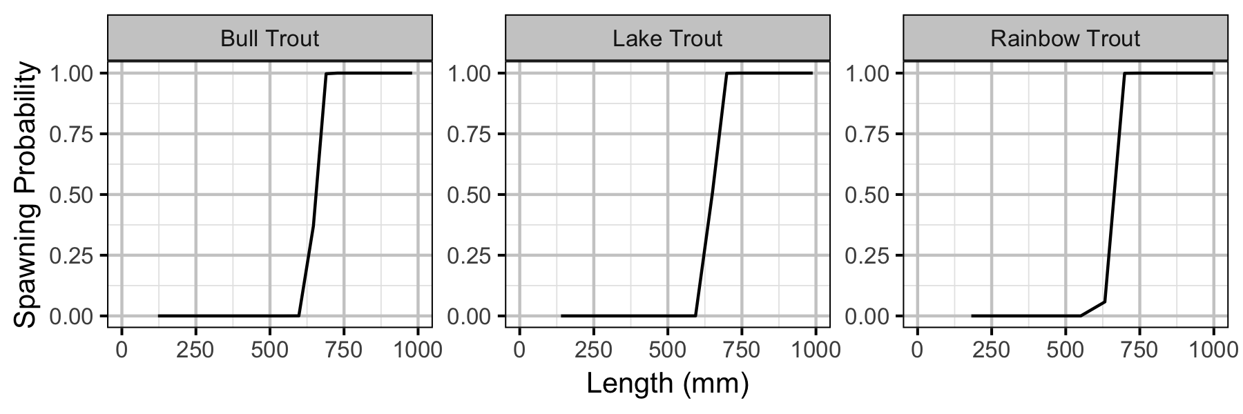
| Ls | 65.0000000 | The length at which 50% mature (cm). | Professional Judgement |
| Sp | 100.0000000 | The maturity (as a function of length) power. | Default |
| es | 1.0000000 | The annual probability of a mature fish spawning. | Default |
| Sm | 0.0000000 | The spawning mortality probability. | Default |
| fb | 1.0000000 | The fecundity (as a function of weight) scaling exponent. | Default |
| tR | 1.0000000 | The age from which survival is density-independent (yr). | Default |
| BH | 1.0000000 | Recruitment follows a Beverton-Holt (1) or Ricker (0) relationship. | Default |
| Rk | 22.9500000 | The lifetime spawners per spawner at low density. | (Chudnow, van Poorten, and McAllister 2018) |
| M | 0.4120817 | The instantaneous mortality rate (per yr). | Current Study |
| Mb | 0.0000000 | The instantaneous mortality rate (as a function of length) scaling exponent. | Default |
| Lv | 50.0000000 | The length at which 50% vulnerable to harvest (cm). | Professional Judgement |
| Vp | 20.0000000 | The vulnerability to harvest (as a function of length) power. | Professional Judgement |
| Llo | 0.0000000 | The lower harvest slot length (cm). | Default |
| Lup | 100.0000000 | The upper harvest slot length (cm). | Default |
| Nc | 0.0000000 | The slot limits non-compliance probability. | Default |
| pi | 0.0691639 | The annual capture probability. | Current Study |
| rho | 0.0000000 | The release probability. | Default |
| Hm | 0.0000000 | The hooking mortality probability. | Default |
| Rmax | 1.0000000 | The number of recruits at the carrying capacity (ind). | Default |
| A0 | 0.0000000 | The initial post age tR density independent mortality probability. | Default |
| Wa | 0.0051027 | The (extrapolated) weight of a 1 cm individual (g). | Current Study |
| fa | 1.0000000 | The (theoretical) fecundity of a 1 g female (eggs). | Default |
| q | 0.1000000 | The catchability (annual probability of capture) for a unit of effort. | Default |
Table 24. Bull Trout yield-per-recruit calculations including the capture probability (pi), exploitation rate (u), and average age, length and weight of fish harvested.
| Type | pi | u | Yield | Age | Length | Weight | Effort |
|---|---|---|---|---|---|---|---|
| actual | 0.0691639 | 0.0691639 | 0.0236255 | 7.270724 | 59.78075 | 2466.607 | 0.6802557 |
| optimal | 0.3440717 | 0.3440717 | 0.0639750 | 6.420277 | 55.96287 | 1940.139 | 4.0024843 |
Lake Trout
Table 25. Lake Trout yield-per-recruit model parameters.
| Parameter | Value | Description | Source |
|---|---|---|---|
| tmax | 30.0000000 | The maximum age (yr). | Professional Judgement |
| k | 0.1500000 | The VB growth coefficient (per yr). | Professional Judgement |
| Linf | 100.0000000 | The VB mean maximum length (cm). | Default |
| t0 | 0.0000000 | The (theoretical) age at zero length (yr). | Default |
| Wb | 3.1754358 | The weight (as a function of length) scaling exponent. | Current Study |
| Ls | 65.0000000 | The length at which 50% mature (cm). | Professional Judgement |
| Sp | 100.0000000 | The maturity (as a function of length) power. | Default |
| es | 1.0000000 | The annual probability of a mature fish spawning. | Default |
| Sm | 0.0000000 | The spawning mortality probability. | Default |
| fb | 1.0000000 | The fecundity (as a function of weight) scaling exponent. | Default |
| tR | 1.0000000 | The age from which survival is density-independent (yr). | Default |
| BH | 1.0000000 | Recruitment follows a Beverton-Holt (1) or Ricker (0) relationship. | Default |
| Rk | 24.1000000 | The lifetime spawners per spawner at low density. | (Myers, Bowen, and Barrowman 1999) |
| M | 0.2147343 | The instantaneous mortality rate (per yr). | Current Study |
| Mb | 0.0000000 | The instantaneous mortality rate (as a function of length) scaling exponent. | Default |
| Lv | 50.0000000 | The length at which 50% vulnerable to harvest (cm). | Professional Judgement |
| Vp | 20.0000000 | The vulnerability to harvest (as a function of length) power. | Professional Judgement |
| Llo | 0.0000000 | The lower harvest slot length (cm). | Default |
| Lup | 100.0000000 | The upper harvest slot length (cm). | Default |
| Nc | 0.0000000 | The slot limits non-compliance probability. | Default |
| pi | 0.0414489 | The annual capture probability. | Current Study |
| rho | 0.0000000 | The release probability. | Default |
| Hm | 0.0000000 | The hooking mortality probability. | Default |
| Rmax | 1.0000000 | The number of recruits at the carrying capacity (ind). | Default |
| A0 | 0.0000000 | The initial post age tR density independent mortality probability. | Default |
| Wa | 0.0053105 | The (extrapolated) weight of a 1 cm individual (g). | Current Study |
| fa | 1.0000000 | The (theoretical) fecundity of a 1 g female (eggs). | Default |
| q | 0.1000000 | The catchability (annual probability of capture) for a unit of effort. | Default |
Table 26. Lake Trout yield-per-recruit calculations including the capture probability (pi), exploitation rate (u), and average age, length and weight of fish harvested.
| Type | pi | u | Yield | Age | Length | Weight | Effort |
|---|---|---|---|---|---|---|---|
| actual | 0.0414489 | 0.0414489 | 0.0710215 | 8.456740 | 68.16605 | 3974.955 | 0.4017864 |
| optimal | 0.2707637 | 0.2707637 | 0.2074532 | 6.498134 | 60.83568 | 2672.363 | 2.9969235 |
Rainbow Trout
Table 27. Rainbow Trout yield-per-recruit model parameters.
| Parameter | Value | Description | Source |
|---|---|---|---|
| tmax | 30.0000000 | The maximum age (yr). | Professional Judgement |
| k | 0.2000000 | The VB growth coefficient (per yr). | Professional Judgement |
| Linf | 100.0000000 | The VB mean maximum length (cm). | Default |
| t0 | 0.0000000 | The (theoretical) age at zero length (yr). | Default |
| Wb | 3.1779885 | The weight (as a function of length) scaling exponent. | Current Study |
| Ls | 65.0000000 | The length at which 50% mature (cm). | Professional Judgement |
| Sp | 100.0000000 | The maturity (as a function of length) power. | Default |
| es | 1.0000000 | The annual probability of a mature fish spawning. | Default |
| Sm | 0.0000000 | The spawning mortality probability. | Default |
| fb | 1.0000000 | The fecundity (as a function of weight) scaling exponent. | Default |
| tR | 1.0000000 | The age from which survival is density-independent (yr). | Default |
| BH | 1.0000000 | Recruitment follows a Beverton-Holt (1) or Ricker (0) relationship. | Default |
| Rk | 12.5000000 | The lifetime spawners per spawner at low density. | (???) |
| M | 0.7159921 | The instantaneous mortality rate (per yr). | Current Study |
| Mb | 0.0000000 | The instantaneous mortality rate (as a function of length) scaling exponent. | Default |
| Lv | 50.0000000 | The length at which 50% vulnerable to harvest (cm). | Professional Judgement |
| Vp | 20.0000000 | The vulnerability to harvest (as a function of length) power. | Professional Judgement |
| Llo | 0.0000000 | The lower harvest slot length (cm). | Default |
| Lup | 100.0000000 | The upper harvest slot length (cm). | Default |
| Nc | 0.0000000 | The slot limits non-compliance probability. | Default |
| pi | 0.1307514 | The annual capture probability. | Current Study |
| rho | 0.0000000 | The release probability. | Default |
| Hm | 0.0000000 | The hooking mortality probability. | Default |
| Rmax | 1.0000000 | The number of recruits at the carrying capacity (ind). | Default |
| A0 | 0.0000000 | The initial post age tR density independent mortality probability. | Default |
| Wa | 0.0056622 | The (extrapolated) weight of a 1 cm individual (g). | Current Study |
| fa | 1.0000000 | The (theoretical) fecundity of a 1 g female (eggs). | Default |
| q | 0.1000000 | The catchability (annual probability of capture) for a unit of effort. | Default |
Table 28. Rainbow Trout yield-per-recruit calculations including the capture probability (pi), exploitation rate (u), and average age, length and weight of fish harvested.
| Type | pi | u | Yield | Age | Length | Weight | Effort |
|---|---|---|---|---|---|---|---|
| actual | 0.1307514 | 0.1307514 | 0.0245374 | 4.574063 | 58.83314 | 2569.316 | 1.329968 |
| optimal | 0.4048375 | 0.4048375 | 0.0479250 | 4.244256 | 56.54300 | 2219.820 | 4.925192 |
Figures
Captures
Sections
Coverage
Detections
Section Use
Condition
Tag Loss
Survival
Yield-per-Recruit
Recommendations
Recommendations include:
- Incorporate recaptures by research crew into survival model.
- Add growth component to survival model to estimate growth parameters and adjust lengths.
- Explore seasonal, annual and length-based variation in natural and fishing mortality.
Acknowledgements
The organisations and individuals whose contributions have made this analysis report possible include:
- Quesnel Lake anglers for reporting their catches
- Habitat Conservation Trust Foundation (HCTF)
- and the anglers, hunters, trappers and guides who contribute to the Trust
- Ministry of Forests, Lands and Natural Resource Operations
- Lee Williston
- Greg Andrusak
- Mike Ramsay
- Reel Adventures
- Kerry Reed
- Vicky Lipinski
References
Bison, Robert, David O’Brien, and Steven J. D. Martell. 2003. “An Analysis of Sustainable Fishing Options for Adams Lake Bull Trout Using Life History and Telemetry Data.” Kamloops, B.C.: BC Ministry of Water Land; Air Protection.
Bradford, Michael J, Josh Korman, and Paul S Higgins. 2005. “Using Confidence Intervals to Estimate the Response of Salmon Populations (Oncorhynchus Spp.) to Experimental Habitat Alterations.” Canadian Journal of Fisheries and Aquatic Sciences 62 (12): 2716–26. https://doi.org/10.1139/f05-179.
Brooks, Steve, Andrew Gelman, Galin L. Jones, and Xiao-Li Meng, eds. 2011. Handbook for Markov Chain Monte Carlo. Boca Raton: Taylor & Francis.
Chudnow, Rachel E., Brett T van Poorten, and Murdoch K. McAllister. 2018. “Estimating Cross-Population Variation in Juvenile Compensation in Survival for Bull Trout (Salvelinus Confluentus): A Bayesian Hierarchical Approach.” Canadian Journal of Fisheries and Aquatic Sciences, November. https://doi.org/10.1139/cjfas-2017-0555.
Fabrizio, Mary C., James D. Nichols, James E. Hines, Bruce L. Swanson, and Stephen T. Schram. 1999. “Modeling Data from Double-Tagging Experiments to Estimate Heterogeneous Rates of Tag Shedding in Lake Trout (Salvelinus Namaycush).” Canadian Journal of Fisheries and Aquatic Sciences 56 (8): 1409–19. http://www.nrcresearchpress.com/doi/pdf/10.1139/f99-069.
He, Ji X., James R. Bence, James E. Johnson, David F. Clapp, and Mark P. Ebener. 2008. “Modeling Variation in Mass-Length Relations and Condition Indices of Lake Trout and Chinook Salmon in Lake Huron: A Hierarchical Bayesian Approach.” Transactions of the American Fisheries Society 137 (3): 801–17. https://doi.org/10.1577/T07-012.1.
Kery, Marc, and Michael Schaub. 2011. Bayesian Population Analysis Using WinBUGS : A Hierarchical Perspective. Boston: Academic Press. http://www.vogelwarte.ch/bpa.html.
Myers, Ransom A., Keith G. Bowen, and Nicholas J. Barrowman. 1999. “Maximum Reproductive Rate of Fish at Low Population Sizes.” Canadian Journal of Fisheries and Aquatic Sciences 56 (12): 2404–19. http://www.nrcresearchpress.com/doi/abs/10.1139/f99-201.
Plummer, Martyn. 2015. “JAGS Version 4.0.1 User Manual.” http://sourceforge.net/projects/mcmc-jags/files/Manuals/4.x/.
R Core Team. 2018. R: A Language and Environment for Statistical Computing. Vienna, Austria: R Foundation for Statistical Computing. https://www.R-project.org/.
Thorley, Joseph L., and Greg F. Andrusak. 2017. “The Fishing and Natural Mortality of Large, Piscivorous Bull Trout and Rainbow Trout in Kootenay Lake, British Columbia (2008–2013).” PeerJ 5 (January): e2874. https://doi.org/10.7717/peerj.2874.