Quesnel Lake Large Trout Natural and Fishing Mortality Analysis 2015
The suggested citation for this analytic report is:
Thorley, J.L. (2016) Quesnel Lake Large Trout Natural and Fishing Mortality Analysis 2015. A Poisson Consulting Analysis Report. URL: https://www.poissonconsulting.ca/f/1323057218.
Background
Quesnel Lake supports recreational fisheries for large Bull Trout, Lake Trout and Rainbow Trout. To provide information on the natural and fishing of large trout, acoustic receivers were deployed at key locations in Quesnel Lake. Large trout were caught by angling and tagged with acoustic transmitters and reward tags.
Methods
Data Preparation
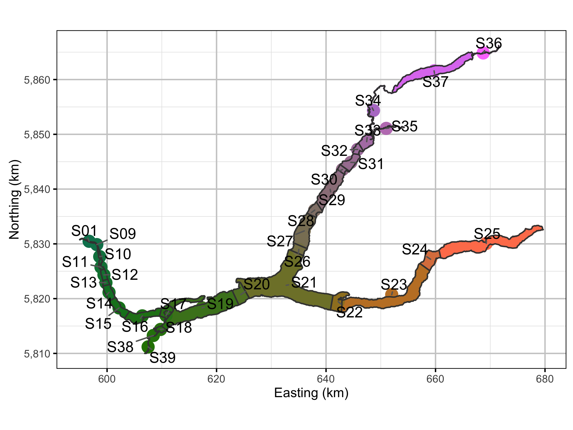
For the purpose of quantifying movement, Quesnel Lake was divided into 32 sections based on the lake morphology and receiver locations. The lake section, acoustic receiver, fish capture and recapture and hourly detection data were provided by Gary Pavan.
The provided data were then converted into an R data package called qlexdatr. During conversion into an R data package:
- Georeferenced information was projected as UTM zone 10N NAD83 (EPSG: 26910).
- Temporal information was converted to Pacific Standard Time (UTC-8).
- If details were not recorded for a specific recapture, it was assumed to have been caught by the public and released and the T-bar tags removed.
- Two or less detections of a fish at a receiver in a given hour were considered unreliable and were discarded.
The hourly receiver detection data in qlexdatr was then resolved into six hour time intervals by section using the make_detect_data function of the lexr R package.
During data resolution:
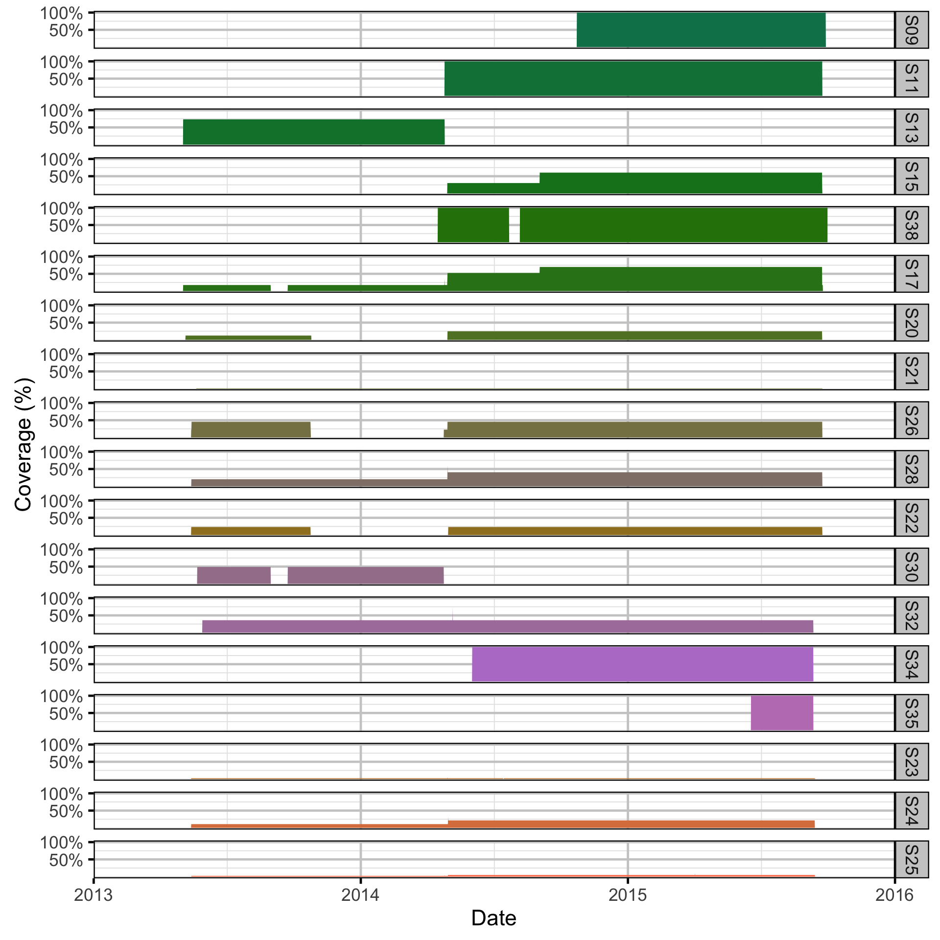
- The proportional receiver coverage at each section in each interval was calculated assuming a detection radius of 500 m, no overlap between receivers and a maximum coverage of 1.
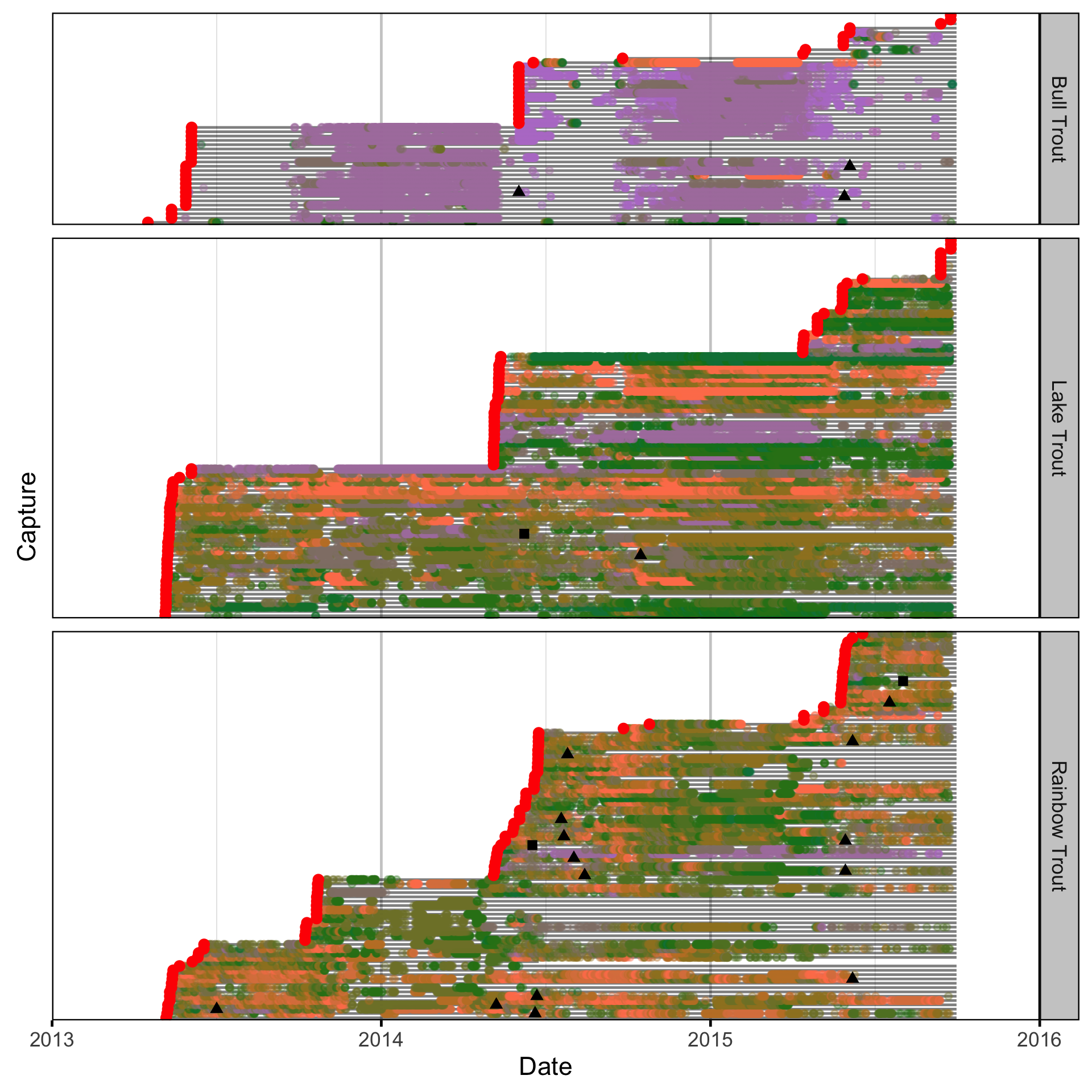
- Each fish was permitted to be in only one section in each time interval. If a fish was detected in more than one section, the section with the most detections was selected. If sections were tied for detections the section with the least receivers was selected. Failing that, the section with the smaller area was selected.
- Each fish was permitted to move between adjacent sections from one interval to the next. If the distance between detections was greater than the number of intervals then the latter detection was considered a jump.
The six hourly sectional detection data were then aggregated into calendar months periods using the make_analysis_data function of the lexr package.
During data aggregation:
- The coverage in each section in each period was the mean coverage across the corresponding time intervals.
- Each fish was permitted to be recaught once in each period. If a fish was recaught twice then the last recapture was chosen.
Statistical Analysis
Hierarchical Bayesian models were fitted to the data using R version 3.2.3 (R Core Team 2015) and JAGS 4.0.1 (Plummer 2015) which interfaced with each other via jaggernaut 2.3.1 (Thorley 2013). For additional information on hierarchical Bayesian modelling in the BUGS language, of which JAGS uses a dialect, the reader is referred to Kery and Schaub (2011, 41–44).
Unless indicated otherwise, the models used prior distributions that were vague in the sense that they did not affect the posterior distributions (Kery and Schaub 2011, 36). The posterior distributions were estimated from a minimum of 1,000 Markov Chain Monte Carlo (MCMC) samples thinned from the second halves of three chains (Kery and Schaub 2011, 38–40). Model convergence was confirmed by ensuring that Rhat (Kery and Schaub 2011, 40) was less than 1.1 for each of the parameters in the model (Kery and Schaub 2011, 61). Model adequacy was confirmed by examination of residual plots.
The posterior distributions of the fixed (Kery and Schaub 2011, 75) parameters are summarised in terms of a point estimate (mean), lower and upper 95% credible limits (2.5th and 97.5th percentiles), the standard deviation (SD), percent relative error (half the 95% credible interval as a percent of the point estimate) and significance (Kery and Schaub 2011, 37, 42).
Variable selection was achieved by dropping insignificant (Kery and Schaub 2011, 37, 42) fixed (Kery and Schaub 2011, 77–82) variables and uninformative random variables. A fixed variables was considered to be insignificant if its significance was \(\geq\) 0.05 while a random variable was considered to be uninformative if its percent relative error was \(\geq\) 80%. The Deviance Information Criterion (DIC) was not used because it is of questionable validity when applied to hierarchical models (Kery and Schaub 2011, 469).
The results are displayed graphically by plotting the modeled relationships between particular variables and the response with 95% credible intervals (CRIs) with the remaining variables held constant. In general, continuous and discrete fixed variables are held constant at their mean and first level values respectively while random variables are held constant at their typical values (expected values of the underlying hyperdistributions) (Kery and Schaub 2011, 77–82). Where informative the influence of particular variables is expressed in terms of the effect size (i.e., percent change in the response variable) with 95% CRIs (Bradford, Korman, and Higgins 2005).
Model Descriptions
Natural and Fishing Mortality
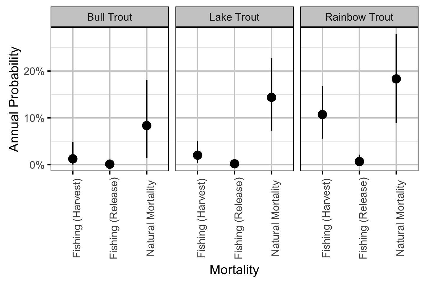
Natural and fishing mortality was estimated from the monthly detection data using a Cormack-Jolly-Seber state-space model (Kery and Schaub 2011, 175–77).
Key assumptions of the mortality model include:
- The probability of an angler reporting a fish with T-bar tags is 90% to 100%.
- The probability of an angler removing the T-bar tags is 90% to 100%.
- The handling mortality is 0 to 20%.
- The annual T-bar tag loss rate is 5 to 10%.
Model Code
The JAGS model code, which uses a series of naming conventions, is presented below.
Natural And Fishing Mortality
| Variable/Parameter | Description |
|---|---|
bAngled |
Annual probability of being recaught |
bDetect |
Interval probability of being detected if inlake |
bHandlingM |
Probability of dying due to (re)capture |
bMove |
Interval probability of moving if alive |
bNaturalM |
Annual probability of dying due to natural causes |
bPublic |
Probability of recapture by public angler (vs research team) |
bReleased[2] |
Probability of a public angler releasing a fish |
bRemoved[2] |
Probability of a public angler removing T-bar tags |
bReported[2] |
Probability of a public angler reporting a T-bar tagged fish |
bTagLoss |
Annual probability of T-bar tag loss |
Natural And Fishing Mortality - Model1
model{

  bDetect ~ dunif(0, 1)
  bMove ~ dunif(0, 1)

  bAngled ~ dunif(0, 1)
  bPublic ~ dunif(0, 1)
  bReported[1] <- 1
  bReported[2] ~ dunif(0.9, 1.0)
  bRemoved[1] <- 0
  bRemoved[2] ~ dunif(0.9, 1)
  bReleased[1] <- 1
  bReleased[2] ~ dunif(0, 1)
  bNaturalM ~ dunif(0, 1)
  bHandlingM ~ dunif(0, 0.2)
  bTagLoss ~ dunif(0.05, 0.1)

  eAngledDaily <- 1-(1-bAngled)^(1/365)
  eNaturalMDaily <- 1-(1-bNaturalM)^(1/365)
  eTagLossDaily <- 1-(1-bTagLoss)^(1/365)

  for (i in 1:nCapture){
    eInlake[i,PeriodCapture[i]] <- 1
    eAlive[i,PeriodCapture[i]] <- 1

    Detected[i,PeriodCapture[i]] ~ dbern(bDetect * eInlake[i,PeriodCapture[i]])
    Moved[i,PeriodCapture[i]] ~ dbern(Detected[i,PeriodCapture[i]] * eAlive[i,PeriodCapture[i]] * bMove)

    eAngled[i,PeriodCapture[i]] ~ dbern((1-(1-eAngledDaily)^Days[PeriodCapture[i]]) * eAlive[i,PeriodCapture[i]])
    Public[i,PeriodCapture[i]] ~ dbern(bPublic)

    eTags[i,PeriodCapture[i]] <- step(sum(Tags[i,PeriodCapture[i],1:2])-1)
    Reported[i,PeriodCapture[i]] ~ dbern(eAngled[i,PeriodCapture[i]] * eTags[i,PeriodCapture[i]] * bReported[Public[i,PeriodCapture[i]]+1])
    Released[i,PeriodCapture[i]] ~ dbern(bReleased[Public[i,PeriodCapture[i]]+1])

    eHandlingM[i,PeriodCapture[i]] <- bHandlingM

    for(j in (PeriodCapture[i]+1):PeriodTagExpire[i]) {
      Removed[i,j-1] ~ dbern(eAngled[i,j-1] * eTags[i,j-1] * bRemoved[Public[i,j-1]+1])
      Tags[i,j,1] ~ dbern(Tags[i,j-1,1] * (1-eTagLossDaily)^Days[j-1] * (1-Removed[i,j-1]))
      Tags[i,j,2] ~ dbern(Tags[i,j-1,2] * (1-eTagLossDaily)^Days[j-1] * (1-Removed[i,j-1]))

      eInlake[i,j] ~ dbern(eInlake[i,j-1] * (1-(eAngled[i,j-1] * (1-Released[i,j-1]))))
      eAlive[i,j] ~ dbern(eInlake[i,j] * eAlive[i,j-1] * (1-eNaturalMDaily)^Days[j-1] * (1 - (eAngled[i,j-1] * Released[i,j-1] * eHandlingM[i,j-1])))

      Detected[i,j] ~ dbern(bDetect * eInlake[i,j])
      Moved[i,j] ~ dbern(Detected[i,j] * eAlive[i,j] * bMove)

      eAngled[i,j] ~ dbern((1-(1-eAngledDaily)^Days[j]) * eAlive[i,j])
      Public[i,j] ~ dbern(bPublic)
      eTags[i,j] <- step(sum(Tags[i,j,1:2])-1)
      Reported[i,j] ~ dbern(eAngled[i,j] * eTags[i,j] * bReported[Public[i,j]+1])
      Released[i,j] ~ dbern(bReleased[Public[i,j]+1])
      eHandlingM[i,j] <- eAngled[i,j] * bHandlingM

    }
  }
}
Results
Due to the preliminary nature of the analysis, the results should be considered preliminary and interpreted with caution for management purposes.
Model Parameters
The posterior distributions for the fixed (Kery and Schaub 2011 p. 75) parameters in each model are summarised below.
Natural And Fishing Mortality - Bull Trout
| Parameter | Estimate | Lower | Upper | SD | Error | Significance |
|---|---|---|---|---|---|---|
| bAngled | 0.05340 | 0.01510 | 0.11570 | 0.02570 | 94 | 0.001 |
| bDetect | 0.49499 | 0.46332 | 0.52744 | 0.01692 | 6 | 0.001 |
| bHandlingM | 0.08950 | 0.00280 | 0.19090 | 0.05590 | 100 | 0.001 |
| bMove | 0.30025 | 0.25490 | 0.34685 | 0.02349 | 15 | 0.001 |
| bNaturalM | 0.08360 | 0.01510 | 0.18080 | 0.04450 | 99 | 0.001 |
| bPublic | 0.23410 | 0.00540 | 0.65930 | 0.19170 | 140 | 0.001 |
| bReleased[1] | 1.00000 | 1.00000 | 1.00000 | 0.00000 | 0 | 0.001 |
| bReleased[2] | 0.53420 | 0.02940 | 0.97840 | 0.29010 | 89 | 0.001 |
| bRemoved[2] | 0.95139 | 0.90262 | 0.99749 | 0.02889 | 5 | 0.001 |
| bReported[1] | 1.00000 | 1.00000 | 1.00000 | 0.00000 | 0 | 0.001 |
| bReported[2] | 0.95017 | 0.90280 | 0.99772 | 0.02931 | 5 | 0.001 |
| bTagLoss | 0.07383 | 0.05115 | 0.09851 | 0.01406 | 32 | 0.001 |
| Convergence | Iterations |
|---|---|
| 1.08 | 10000 |
Natural And Fishing Mortality - Lake Trout
| Parameter | Estimate | Lower | Upper | SD | Error | Significance |
|---|---|---|---|---|---|---|
| bAngled | 0.02588 | 0.00561 | 0.05922 | 0.01400 | 100 | 0.001 |
| bDetect | 0.83534 | 0.81670 | 0.85365 | 0.00943 | 2 | 0.001 |
| bHandlingM | 0.09280 | 0.00500 | 0.19370 | 0.05700 | 100 | 0.001 |
| bMove | 0.68859 | 0.65982 | 0.71729 | 0.01472 | 4 | 0.001 |
| bNaturalM | 0.14420 | 0.07390 | 0.22730 | 0.03990 | 53 | 0.001 |
| bPublic | 0.79100 | 0.43930 | 0.99520 | 0.16960 | 35 | 0.001 |
| bReleased[1] | 1.00000 | 1.00000 | 1.00000 | 0.00000 | 0 | 0.001 |
| bReleased[2] | 0.49350 | 0.09790 | 0.90960 | 0.21750 | 82 | 0.001 |
| bRemoved[2] | 0.95165 | 0.90312 | 0.99782 | 0.02899 | 5 | 0.001 |
| bReported[1] | 1.00000 | 1.00000 | 1.00000 | 0.00000 | 0 | 0.001 |
| bReported[2] | 0.95107 | 0.90277 | 0.99707 | 0.02867 | 5 | 0.001 |
| bTagLoss | 0.07331 | 0.05106 | 0.09842 | 0.01415 | 32 | 0.001 |
| Convergence | Iterations |
|---|---|
| 1.07 | 20000 |
Natural And Fishing Mortality - Rainbow Trout
| Parameter | Estimate | Lower | Upper | SD | Error | Significance |
|---|---|---|---|---|---|---|
| bAngled | 0.14670 | 0.08790 | 0.21640 | 0.03280 | 44 | 0.001 |
| bDetect | 0.60447 | 0.57992 | 0.62940 | 0.01241 | 4 | 0.001 |
| bHandlingM | 0.06340 | 0.00160 | 0.17930 | 0.04980 | 140 | 0.001 |
| bMove | 0.84495 | 0.82145 | 0.86869 | 0.01236 | 3 | 0.001 |
| bNaturalM | 0.18350 | 0.09260 | 0.28000 | 0.04880 | 51 | 0.001 |
| bPublic | 0.73240 | 0.50070 | 0.89790 | 0.10060 | 27 | 0.001 |
| bReleased[1] | 1.00000 | 1.00000 | 1.00000 | 0.00000 | 0 | 0.001 |
| bReleased[2] | 0.80520 | 0.58910 | 0.95470 | 0.09790 | 23 | 0.001 |
| bRemoved[2] | 0.91152 | 0.90037 | 0.93840 | 0.01035 | 2 | 0.001 |
| bReported[1] | 1.00000 | 1.00000 | 1.00000 | 0.00000 | 0 | 0.001 |
| bReported[2] | 0.95927 | 0.90530 | 0.99837 | 0.02834 | 5 | 0.001 |
| bTagLoss | 0.07330 | 0.05105 | 0.09843 | 0.01403 | 32 | 0.001 |
| Convergence | Iterations |
|---|---|
| 1.08 | 10000 |
Figures
Spatial Data


Natural And Fishing Mortality

Acknowledgements
The organisations and individuals whose contributions have made this analysis report possible include:
- Quesnel Lake anglers for reporting their catches
- Habitat Conservation Trust Foundation (HCTF) and the anglers, hunters, trappers and guides who contribute to the Trust
- Ministry of Forests, Lands and Natural Resource Operations (MFLNRO)
- Lee Williston
- Mike Ramsay
- Redfish Consulting
- Greg Andrusak
- Harvey Andrusak
- Reel Adventures
- Kerry Reed
- Gary Pavan
- Vicky Lipinski
- Bernhard Konrad
References
Bradford, Michael J, Josh Korman, and Paul S Higgins. 2005. “Using Confidence Intervals to Estimate the Response of Salmon Populations (Oncorhynchus Spp.) to Experimental Habitat Alterations.” Canadian Journal of Fisheries and Aquatic Sciences 62 (12): 2716–26. https://doi.org/10.1139/f05-179.
Kery, Marc, and Michael Schaub. 2011. Bayesian Population Analysis Using WinBUGS : A Hierarchical Perspective. Boston: Academic Press. http://www.vogelwarte.ch/bpa.html.
Plummer, Martyn. 2015. “JAGS Version 4.0.1 User Manual.” http://sourceforge.net/projects/mcmc-jags/files/Manuals/4.x/.
R Core Team. 2015. “R: A Language and Environment for Statistical Computing.” Vienna, Austria: R Foundation for Statistical Computing. http://www.R-project.org/.
Thorley, J. L. 2013. “Jaggernaut: An R Package to Facilitate Bayesian Analyses Using JAGS (Just Another Gibbs Sampler).” Nelson, B.C.: Poisson Consulting Ltd. https://github.com/poissonconsulting/jaggernaut.