Cowichan Lake Cuththroat Trout Exploitation Analysis 2023
The suggested citation for this analytic appendix is:
Dalgarno, S. & Thorley, J.L. (2024) Cowichan Lake Cuththroat Trout Exploitation Analysis 2023. A Poisson Consulting Analysis Appendix. URL: https://www.poissonconsulting.ca/f/1638637752.
Background
Cowichan Lake supports an important Cutthroat Trout fishery. To provide information on the natural and fishing mortality, Cutthroat Trout were caught by angling and tagged with acoustic transmitters and/or a $100 reward tag. Some acoustic transmitters were equipped with depth and temperature sensors.
A fixed receiver array was deployed in the lake to monitor fish movements and location year-round. Additional fixed receivers were deployed during the spawning season at known spawning tributaries. A lake census was completed 4 times per year using mobile receivers.
The objectives of this analysis are to:
- Estimate fishing and natural mortality.
- Estimate annual variation in fishing and natural mortality.
- Estimate seasonal variation in fishing and natural mortality.
- Estimate effect of handling on natural mortality.
- Estimate variation in fishing and natural mortality by fork length.
- Estimate spawning probability.
- Estimate variation in spawning probability by fork length.
- Estimate spawning mortality.
Data Preparation
The data were provided to Poisson Consulting Ltd. by Aswea Porter following extensive data screening.
Statistical Analysis
Model parameters were estimated using Bayesian methods. The estimates were produced using JAGS (Plummer 2003). For additional information on Bayesian estimation the reader is referred to McElreath (2020).
Unless stated otherwise, the Bayesian analyses used weakly informative normal and half-normal prior distributions (Gelman, Simpson, and Betancourt 2017). The posterior distributions were estimated from 1500 Markov Chain Monte Carlo (MCMC) samples thinned from the second halves of 3 chains (Kery and Schaub 2011, 38–40). Model convergence was confirmed by ensuring that the potential scale reduction factor \(\hat{R} \leq 1.05\) (Kery and Schaub 2011, 40) and the effective sample size (Brooks et al. 2011) \(\textrm{ESS} \geq 150\) for each of the monitored parameters (Kery and Schaub 2011, 61).
The parameters are summarised in terms of the point estimate, lower and upper 95% credible limits (CLs) and the surprisal s-value (Greenland 2019). The estimate is the median (50th percentile) of the MCMC samples while the 95% CLs are the 2.5th and 97.5th percentiles. The s-value indicates how surprising it would be to discover that the true value of the parameter is in the opposite direction to the estimate (Greenland 2019). An s-value of \(>\) 4.3 bits, which is equivalent to a significant p-value \(<\) 0.05 (Kery and Schaub 2011; Greenland and Poole 2013), indicates that the surprise would be equivalent to throwing at least 4.3 heads in a row.
The condition that parameters describing the effects of secondary (nuisance) explanatory variable(s) have significant p-values was used as a model selection heuristic (Kery and Schaub 2011). Based on a similar argument, the condition that random effects have a standard deviation with a lower 95% CL \(>\) 5% of the estimate was used as an additional model selection heuristic. Primary explanatory variables are evaluated based on their estimated effect sizes with 95% CLs (Bradford, Korman, and Higgins 2005)
The results are displayed graphically by plotting the modeled relationships between particular variables and the response(s) with the remaining variables held constant. In general, continuous and discrete fixed variables are held constant at their mean and first level values, respectively, while random variables are held constant at their typical values (expected values of the underlying hyperdistributions) (Kery and Schaub 2011, 77–82).
The analyses were implemented using R version 4.3.3
(R Core Team 2021) and the
mbr family of packages.
Model Descriptions
Survival
The natural mortality and recapture probability were estimated using a Bayesian individual state-space survival model (Thorley and Andrusak 2017) with monthly intervals. The survival model incorporated natural, handling and spawning mortality, acoustic detections and movements from a fixed receiver array and quarterly lake census, vertical movements from acoustic tags equipped with depth sensors, FLOY tag loss, recapture, reporting and release.
The expected fork length at monthly period \(t\) was estimated from length
at capture (\(L_{i,fi}\)) plus the length increment expected under a Von
Bertalanffy Growth Curve (Walters and Martell 2004)
\[L_{i,t} = L_{i,fi} + (L_{∞} − L_{i,fi} )(1 − e^{(−\frac{1}{12} \cdot k(t −fi))})\]
where \(fi\) is the period at capture and the \(\frac{1}{12}\) exponent
adjusts for the fact that there are 12 periods per year.Linf was fixed
to a biologically plausible value of 775 mm based on prior information
(personal communication, R. Ptolemy); k of 0.23 was estimated from 88
aged Cutthroat Trout in Cowichan Lake (personal communication, Brendan
Andersen).
The probability of spawning at estimated fork length \(L\) is determined by
\[S = \frac{L^{S_p}}{L_s^{S_p} + L^{S_p}} \cdot {E_s}\]
where \(L_s\) is the length at which 50% of fish are mature, \(E_s\) is the probability of a mature fish spawning and \(S_p\) is the maturity (as a function of length) power.
Additional key assumptions of the survival model include all but two of the assumptions in Thorley and Andrusak (2017) – the exceptions being 3 (no loss of FLOY tags) and 11 (anglers report all FLOY tags). The survival model also assumes that:
- The monthly interval probability of FLOY tag loss is 0.001.
- All recaptured fish that are released have their FLOY tags removed.
- Reporting of a recaptured fish with a FLOY tag is likely greater
than 90%.
- The effect of handling mortality is restricted to the first two
monthly periods after initial capture or recapture.
- The effect of spawning mortality is restricted to the spawning
period.
- Acoustic tags are functional over their estimated battery lifespan
and are not shed.
- Recapture probability varies by month and size class.
- Natural mortality varies by month, study year and size class.
- The probability of detection depends on whether a fish is alive or has died near or far from a receiver and whether a census has occurred.
Study years span from October 01 to September 30 of the following year (i.e., study year 1 is 2019-10-01 to 2020-09-30). Since data collection started in October, use of study year instead of calendar year ensured that all months were represented in each year. Observations after study year 4 (i.e., in October 2023) were removed from this year’s analysis.
Size classes are defined as small (\(\le\) 350 mm), medium (351 \(-\) 500 mm) and large (> 500 mm). Size class membership can change in each period depending on the fork length predicted by the growth model.
Preliminary analyses indicated lack of support for variation in recapture probability and spawning probability by study year.
We assumed that the monthly interval probability of FLOY tag loss was 0.001 (0.012 annual probability) based on tag loss estimates from double-tagged Lake Trout in Horse Lake.
Preliminary attempts to estimate tag loss in the model using an uninformative prior confirmed that this assumption was consistent with the available information, although we had to fix tag loss in the model to avoid poor convergence.
We assumed that fish detected in monitored spawning tributaries represents all spawning tagged fish in the lake. The ‘spawning window’ was defined as February to May given that there was consistent receiver coverage in spawning tributaries across years. Receivers were also placed in spawning tributaries in January in study years 3 and 4. Four fish that were detected in a spawning tributary only in January (all in study year 4) were not assigned a status of ‘spawning’. Two study years had partial coverage in February (starting Feb 10-11 and Feb 17-19). These spawning detections were included because we assumed that most spawning events would occur toward the end of the month.
Model Templates
Survival
.model{
  bMortality ~ dnorm(-3, 3^-2)
  bMortalityHandling ~ dnorm(0, 2^-2)
  bMonthsHandling <- 2
  bMortalitySpawning ~ dnorm(0, 2^-2)
  bLs ~  dunif(100, 1000)
  bSp ~ dexp(1/20)
  bEs ~ dbeta(1,1)

  bDetectedAlive ~ dbeta(1, 1)
  bDieNear ~ dbeta(1, 1)
  bDetectedDeadNear ~ dbeta(10, 1)
  bDetectedDeadFar ~ dbeta(1, 10)
  bDetectedCensus ~ dbeta(1, 1)
  bMovedH ~ dbeta(1, 1)
  bMovedV ~ dbeta(1, 1)
  bRecaptured ~ dnorm(0, 2^-2)
  bReported ~ dbeta(1, 1)
  bReleased ~ dbeta(1, 1)
  bTagLoss <- 0.001

  bMortalityAnnual[1] <- 0
  for (i in 2:nAnnual) {
    bMortalityAnnual[i] ~ dnorm(0, 2^-2)
  }
  bRecapturedSize[1] <- 0
  for (i in 2:nSize) {
    bRecapturedSize[i] ~ dnorm(0, 2^-2)
  }
  bMortalitySize[1] <- 0
  for (i in 2:nSize) {
    bMortalitySize[i] ~ dnorm(0, 2^-2)
  }
  sRecapturedMonth ~ dexp(1)
  for (i in 1:nMonth) {
    bRecapturedMonth[i] ~ dnorm(0, sRecapturedMonth^-2)
  }
  sMortalityMonth ~ dexp(1)
  for (i in 1:nMonth) {
    bMortalityMonth[i] ~ dnorm(0, sMortalityMonth^-2)
  }
  for (i in 1:nCapture){
    eMortalityHandling[i, PeriodCapture[i]] <- ilogit(bMortalityHandling)
    eMonthsSinceCapture[i,PeriodCapture[i]] <- 1-Recaptured[i,PeriodCapture[i]]
    eMortalitySpawning[i, PeriodCapture[i]] <- ilogit(bMortalitySpawning) * SpawningPeriod[PeriodCapture[i]]

    eDetectedAlive[i] <- bDetectedAlive
    eDieNear[i] ~ dbern(bDieNear)
    eDetectedDeadNear[i] <- bDetectedDeadNear
    eDetectedDeadFar[i] <- bDetectedDeadFar
    eDetectedDead[i] <- eDieNear[i] * eDetectedDeadNear[i] +
      (1 - eDieNear[i]) * eDetectedDeadFar[i]

    logit(eMortality[i,PeriodCapture[i]]) <- bMortality + bMortalityAnnual[Annual[PeriodCapture[i]]] + bMortalitySize[Size[i, PeriodCapture[i]]] + bMortalityMonth[Month[PeriodCapture[i]]]

    eMovedH[i,PeriodCapture[i]] <- bMovedH
    eMovedV[i,PeriodCapture[i]] <- bMovedV
    eDetected[i,PeriodCapture[i]] <- Alive[i,PeriodCapture[i]] * eDetectedAlive[i] +
      (1-Alive[i,PeriodCapture[i]]) * eDetectedDead[i]
    eDetectedCensus[i,PeriodCapture[i]] <- bDetectedCensus
    logit(eRecaptured[i,PeriodCapture[i]]) <- bRecaptured + bRecapturedMonth[Month[PeriodCapture[i]]] + bRecapturedSize[Size[i,PeriodCapture[i]]]
    eReported[i,PeriodCapture[i]] <- bReported
    eReleased[i,PeriodCapture[i]] <- bReleased

    InLake[i,PeriodCapture[i]] <- 1
    Alive[i,PeriodCapture[i]] <- 1
    TBarTag[i,PeriodCapture[i]] ~ dbern(1-bTagLoss)

    Detected[i,PeriodCapture[i]] ~ dbern(Monitored[i,PeriodCapture[i]] * eDetected[i,PeriodCapture[i]])
    DetectedCensus[i,PeriodCapture[i]] ~ dbern(InLake[i,PeriodCapture[i]] * Monitored[i,PeriodCapture[i]] * eDetectedCensus[i,PeriodCapture[i]] * Census[PeriodCapture[i]])
    MovedH[i,PeriodCapture[i]] ~ dbern(Alive[i,PeriodCapture[i]] * Detected[i,PeriodCapture[i]] * eMovedH[i,PeriodCapture[i]])
    MovedV[i,PeriodCapture[i]] ~ dbern(Alive[i,PeriodCapture[i]] * Sensor[i,PeriodCapture[i]] * Detected[i,PeriodCapture[i]] * eMovedV[i,PeriodCapture[i]])

    Recaptured[i,PeriodCapture[i]] ~ dbern(Alive[i,PeriodCapture[i]] * eRecaptured[i,PeriodCapture[i]])
    Reported[i,PeriodCapture[i]] ~ dbern(Recaptured[i,PeriodCapture[i]] * eReported[i,PeriodCapture[i]] * TBarTag[i,PeriodCapture[i]])
    Released[i,PeriodCapture[i]] ~ dbern(Recaptured[i,PeriodCapture[i]] * eReleased[i,PeriodCapture[i]])

    for(a in (AnnualCapture[i]):nAnnual){
      eSpawning[i,a] <- (((LengthSpawned[i,a]^bSp) / (bLs^bSp + LengthSpawned[i,a]^bSp)) * bEs)
    }
  for(j in (PeriodCapture[i]+1):nPeriod) {

    eMortalityHandling[i,j] <- ilogit(bMortalityHandling) * step(bMonthsHandling - eMonthsSinceCapture[i,j-1] - 1)
    eMonthsSinceCapture[i,j] <- (1-Recaptured[i,j]) * (eMonthsSinceCapture[i,j-1] + 1)
    eMortalitySpawning[i,j] <- ilogit(bMortalitySpawning) * Spawned[i,j]
    logit(eMortality[i,j]) <- bMortality + bMortalityAnnual[Annual[j]] + bMortalitySize[Size[i, j]] * (1 - Spawned[i,j]) + bMortalityMonth[Month[j]] * (1 - Spawned[i,j])
    Spawned[i,j] ~ dbern(Monitored[i,j] * SpawningPeriod[j] * eSpawning[i,Annual[j]])

    eDetected[i,j] <- Alive[i,j] * eDetectedAlive[i] + (1-Alive[i,j]) * eDetectedDead[i]
    eDetectedCensus[i,j] <- bDetectedCensus

    eMovedH[i,j] <- bMovedH
    eMovedV[i,j] <- bMovedV
    logit(eRecaptured[i,j]) <-  bRecaptured + bRecapturedMonth[Month[j]] + bRecapturedSize[Size[i,j]]
    eReported[i,j] <- bReported
    eReleased[i,j] <- bReleased

    InLake[i,j] ~ dbern(InLake[i,j-1] * ((1 - (Recaptured[i,j-1])) + Recaptured[i,j-1] * Released[i,j-1]))
    Alive[i,j] ~ dbern(InLake[i,j] * Alive[i,j-1] * (1-eMortality[i,j-1]) * (1-eMortalityHandling[i,j-1]) * (1-eMortalitySpawning[i,j-1]))
    TBarTag[i,j] ~ dbern(TBarTag[i,j-1] * (1-Recaptured[i,j-1]) * (1-bTagLoss))

    Detected[i,j] ~ dbern(InLake[i,j] * Monitored[i,j] * eDetected[i,j])
    DetectedCensus[i,j] ~ dbern(InLake[i,j] * Monitored[i,j] * eDetectedCensus[i,j] * Census[j])
    MovedH[i,j] ~ dbern(Alive[i,j-1] * Monitored[i,j] * eMovedH[i,j])
    MovedV[i,j] ~ dbern(Alive[i,j] * Sensor[i,j] * Monitored[i,j] * eMovedV[i,j])

    Recaptured[i,j] ~ dbern(Alive[i,j] * eRecaptured[i,j])
    Reported[i,j] ~ dbern(Recaptured[i,j] * eReported[i,j] * TBarTag[i,j])
    Released[i,j] ~ dbern(Recaptured[i,j] * eReleased[i,j])
  }
  }
Block 1. Survival model description.
Results
Tables
Survival
Table 1. Parameter descriptions.
| Parameter | Description |
|---|---|
bDetectedAlive |
Probability of being detected by a fixed receiver if alive |
bDetectedCensus |
Probability of being detected by a mobile receiver during a census period |
bDetectedDeadFar |
Probability of being detected if dead far from a fixed receiver |
bDetectedDeadNear |
Probability of being detected if dead near to a fixed receiver |
bDieNear |
Probability of dying near to (vs far from) a fixed receiver |
bEs |
The annual probability of a mature fish spawning |
bLs |
The length at which 50% of fish mature. |
bMonthsHandling |
The number of months for which handling affects mortality. |
bMortalityAnnual[i] |
Effect of ith study year on bMortality |
bMortalityHandling |
Log odds probability of dying after (re)capture in a monthly period. |
bMortalityMonth[i] |
Effect of ith month on bMortality |
bMortalitySize[i] |
Effect of ith size class on bMortality |
bMortalitySpawning |
Log odds probability of dying after spawning in a monthly period. |
bMortality |
Log odds probability of dying of natural causes in a monthly period in the 1st season of the 1st study year |
bMovedH |
Probability of moving horizontally if alive and detected in a monthly period |
bMovedV |
Probability of moving vertically if alive and detected in a monthly period |
bRecapturedMonth[i] |
Effect of ith month on bRecaptured |
bRecapturedSize[i] |
Effect of ith size class on bRecaptured |
bRecaptured |
Log odds probability of being recaptured if alive in a monthly period |
bReleased |
Probability of being released if recaptured |
bReported |
Probability of being reported if recaptured with a FLOY tag |
bSp |
The maturity (as a function of length) power |
sMortalityMonth |
Standard deviation of the random effect of
bMortalityMonth |
sRecapturedMonth |
Standard deviation of the random effect of
bRecapturedMonth |
Table 2. Model coefficients.
| term | estimate | lower | upper | svalue |
|---|---|---|---|---|
| bDetectedAlive | 0.8375755 | 0.8210177 | 0.8533005 | 10.551708 |
| bDetectedCensus | 0.2702202 | 0.2402739 | 0.3053491 | 10.551708 |
| bDetectedDeadFar | 0.0094250 | 0.0050473 | 0.0156601 | 10.551708 |
| bDetectedDeadNear | 0.9727015 | 0.9500951 | 0.9882297 | 10.551708 |
| bDieNear | 0.1737226 | 0.1156306 | 0.2454140 | 10.551708 |
| bEs | 0.2428071 | 0.2083370 | 0.2829326 | 10.551708 |
| bLs | 407.9968075 | 392.0481766 | 422.5025806 | 10.551708 |
| bMortality | -2.7568576 | -3.7142054 | -2.1080086 | 10.551708 |
| bMortalityAnnual[2] | -0.6255056 | -1.3414411 | 0.0440292 | 3.922352 |
| bMortalityAnnual[3] | -0.7645928 | -1.3999920 | -0.1520198 | 5.796821 |
| bMortalityAnnual[4] | 0.3050115 | -0.2257240 | 0.8367744 | 1.820389 |
| bMortalityHandling | -3.1992778 | -4.8929420 | -2.5421481 | 10.551708 |
| bMortalitySize[2] | -0.2536786 | -0.7361078 | 0.2431523 | 1.635829 |
| bMortalitySize[3] | 0.7534943 | 0.1446327 | 1.4163236 | 5.693727 |
| bMortalitySpawning | -1.9172027 | -2.6785626 | -1.3887909 | 10.551708 |
| bMovedH | 0.5812060 | 0.5603906 | 0.6007258 | 10.551708 |
| bMovedV | 0.5006144 | 0.4492197 | 0.5534175 | 10.551708 |
| bRecaptured | -4.9707351 | -5.8107138 | -4.2491255 | 10.551708 |
| bRecapturedSize[2] | 0.8362891 | 0.1445183 | 1.6479300 | 5.907852 |
| bRecapturedSize[3] | 1.4332053 | 0.5753343 | 2.3031767 | 8.966746 |
| bReleased | 0.4460089 | 0.3223654 | 0.5844766 | 10.551708 |
| bReported | 0.9885818 | 0.9317024 | 0.9996544 | 10.551708 |
| bSp | 16.8428520 | 12.0407090 | 22.9989434 | 10.551708 |
| sMortalityMonth | 0.7897345 | 0.2619868 | 1.7048814 | 10.551708 |
| sRecapturedMonth | 0.5277492 | 0.1083606 | 1.1209293 | 10.551708 |
Table 3. Model convergence.
| n | K | nchains | niters | nthin | ess | rhat | converged |
|---|---|---|---|---|---|---|---|
| 13824 | 25 | 3 | 500 | 30 | 189 | 1.038 | TRUE |
Table 4. The estimated annual interval probabilities (with 95% CIs). ‘Natural Mortality’ is the natural mortality averaged across study year and the three size classes for a non-spawning fish. ‘Natural Mortality Spawned’ is the natural mortality for a fish that spawns. ‘Spawning Mortality’ is the probability of mortality from spawning, assuming that the effect of spawning lasts for fourth months (i.e., the spawning window). ‘Handling Mortality’ is the probability of mortality from handling, assuming that the effect of handling lasts for two months and occurs once in a year. ‘Release’ is the probability of being released if recaptured. ‘Recapture’ is the probability of recapture as the average of the three size classes. ‘Harvest Mortality’ is the recapture probability multiplied by the probability of being harvested if recaptured, assuming that recapture can only occur once in a year.
| derived quantity | estimate | lower | upper |
|---|---|---|---|
| Natural Mortality | 0.5600 | 0.4890 | 0.628 |
| Natural Mortality Spawned | 0.7480 | 0.6540 | 0.823 |
| Spawning Mortality | 0.4220 | 0.2330 | 0.590 |
| Handling Mortality | 0.0768 | 0.0148 | 0.141 |
| Release | 0.4460 | 0.3220 | 0.584 |
| Recapture | 0.1970 | 0.1440 | 0.258 |
| Harvest Mortality | 0.1080 | 0.0715 | 0.152 |
Spawning
Table 5. The estimated parameters from the spawning by fork length sub-model. ‘Es’ is the probability of a mature fish spawning. ‘Ls’ is the fork length (mm) at which 50% of fish are mature. ‘Sp’ is the maturity power (as a function of fork length).
| derived quantity | estimate | lower | upper |
|---|---|---|---|
| Es | 0.243 | 0.208 | 0.283 |
| Ls | 408.000 | 392.000 | 423.000 |
| Sp | 16.800 | 12.000 | 23.000 |
Figures
Growth
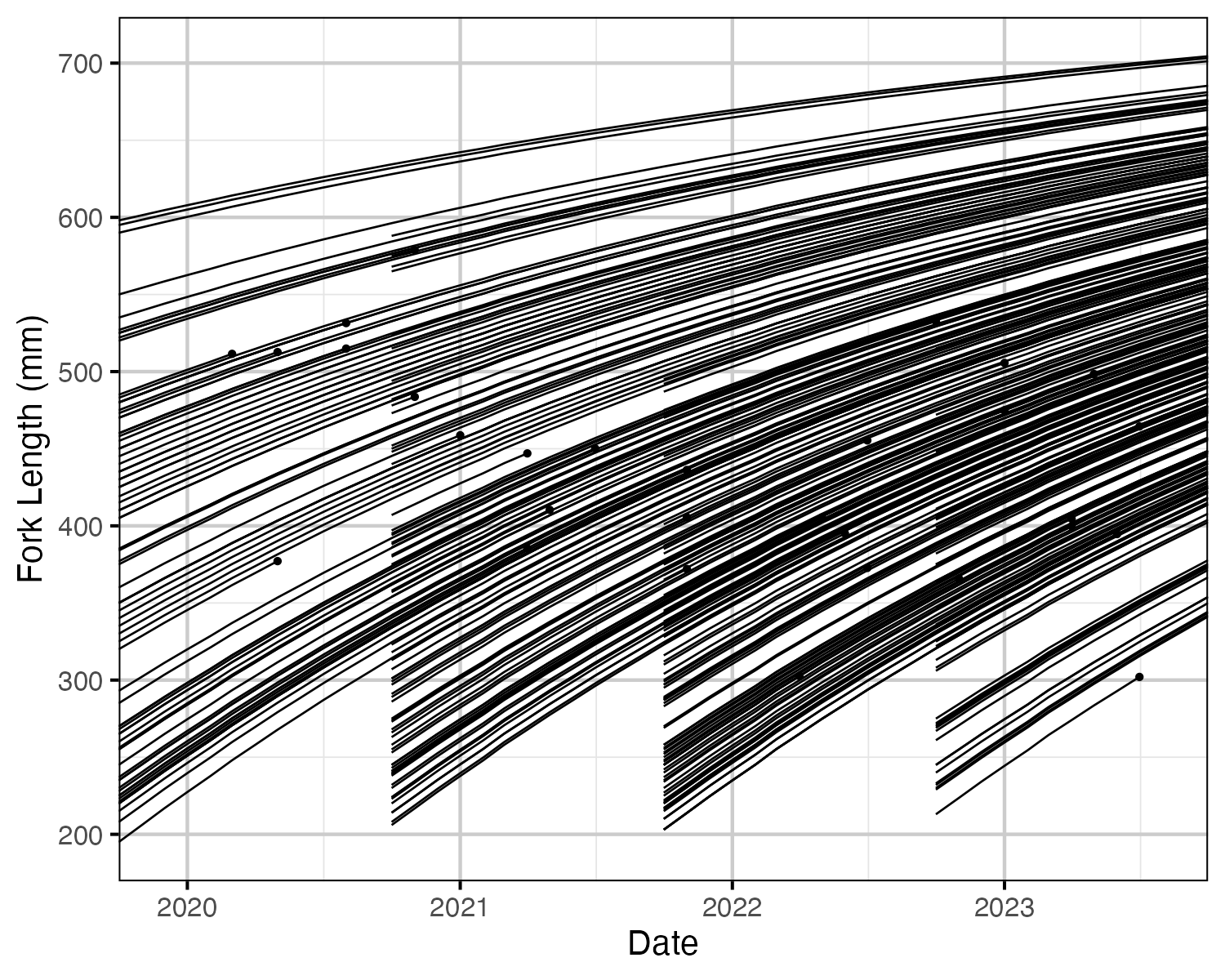
Figure 1. Estimated fork length for each fish by date. Points represent recapture and harvest.
Survival
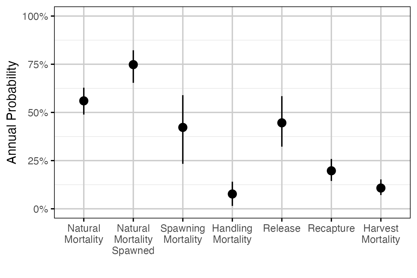
Figure 2. The estimated annual interval probabilities (with 95% CIs). ‘Natural Mortality’ is the natural mortality averaged across study year and the three size classes for a non-spawning fish. ‘Natural Mortality Spawned’ is the natural mortality for a fish that spawns. ‘Spawning Mortality’ is the probability of mortality from spawning, assuming that the effect of spawning lasts for fourth months (i.e., the spawning window). ‘Handling Mortality’ is the probability of mortality from handling, assuming that the effect of handling lasts for two months and occurs once in a year. ‘Release’ is the probability of being released if recaptured. ‘Recapture’ is the probability of recapture as the average of the three size classes. ‘Harvest Mortality’ is the recapture probability multiplied by the probability of being harvested if recaptured, assuming that recapture can only occur once in a year.
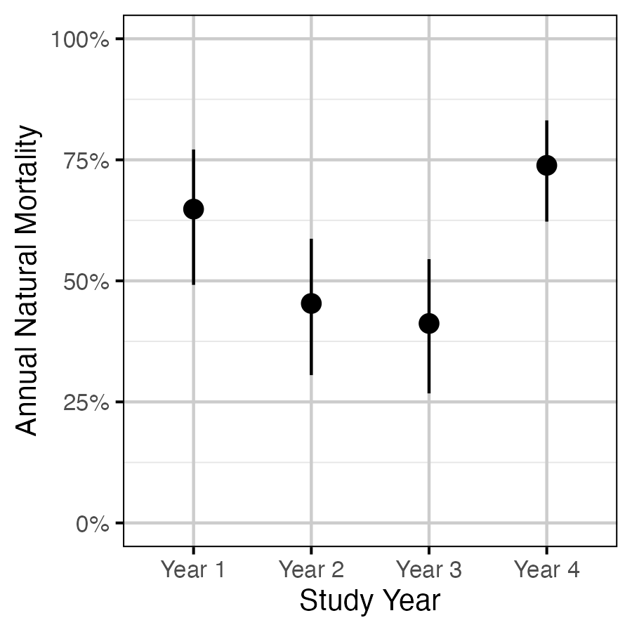
Figure 3. The estimated annual natural mortality by study year averaged across size class for a non-spawning fish (with 95% CIs).
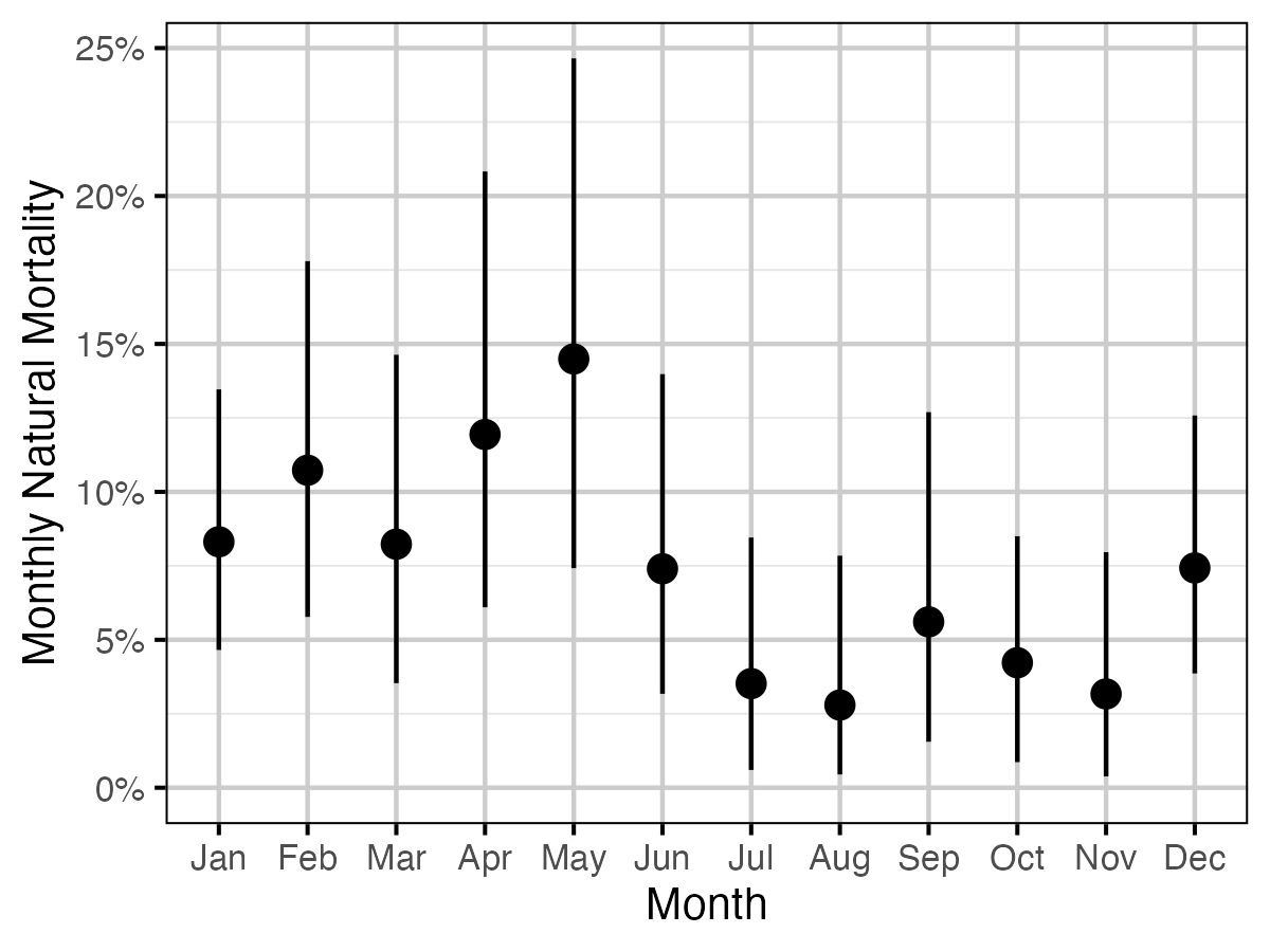
Figure 4. The estimated monthly natural mortality averaged across study year and size class for a non-spawning fish (with 95% CIs).
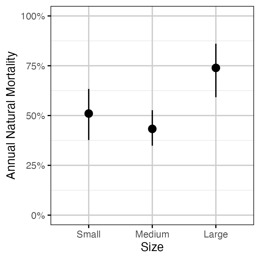
Figure 5. The estimated annual natural mortality by size class, averaged across study year for a non-spawning fish (with 95% CIs). Size classes are defined as small (<= 350 mm), medium (351 - 500 mm) and large (> 500 mm).
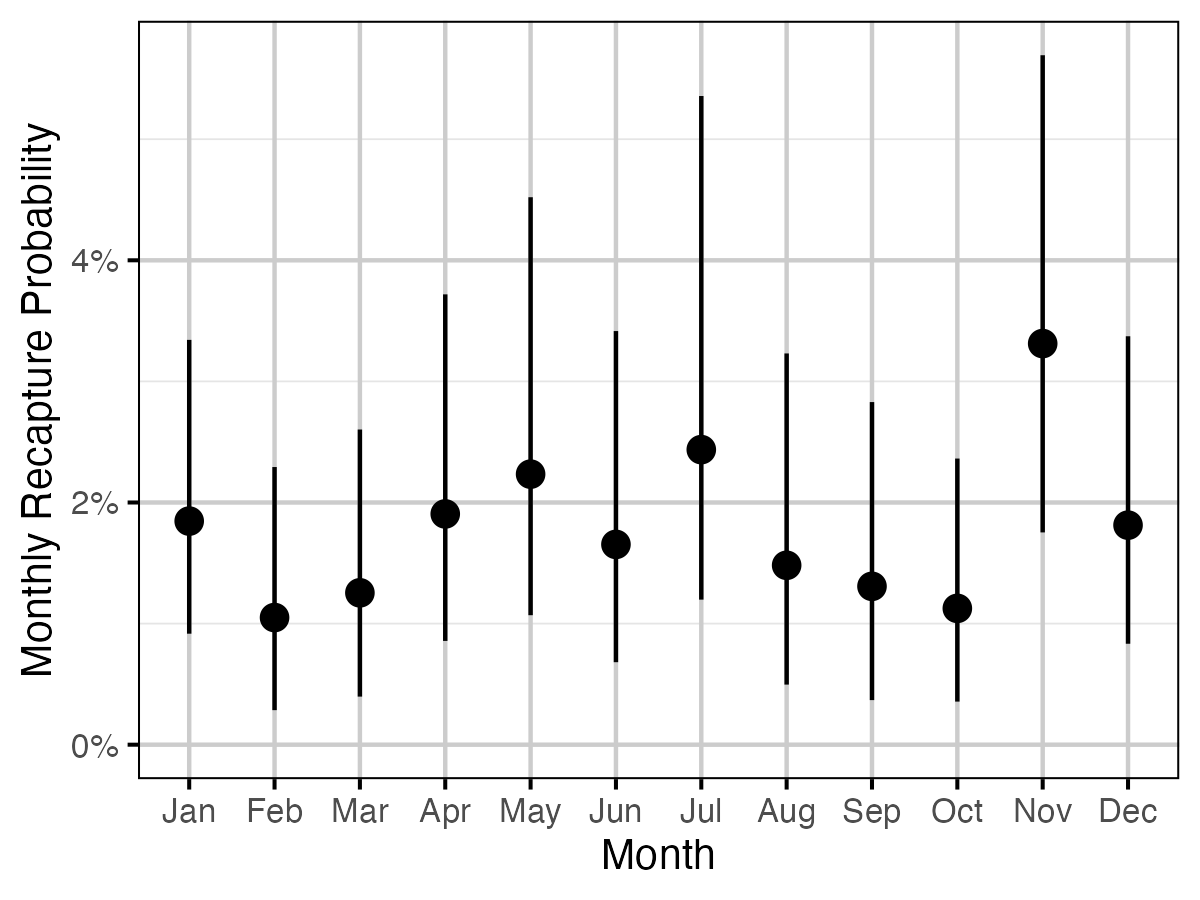
Figure 6. The estimated monthly recapture probability averaged across size class (with 95% CIs).
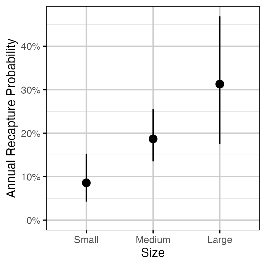
Figure 7. The estimated annual recapture probability by size class (with 95% CIs). Size classes are defined as small (<= 350 mm), medium (351 - 500 mm) and large (> 500 mm).
Spawning
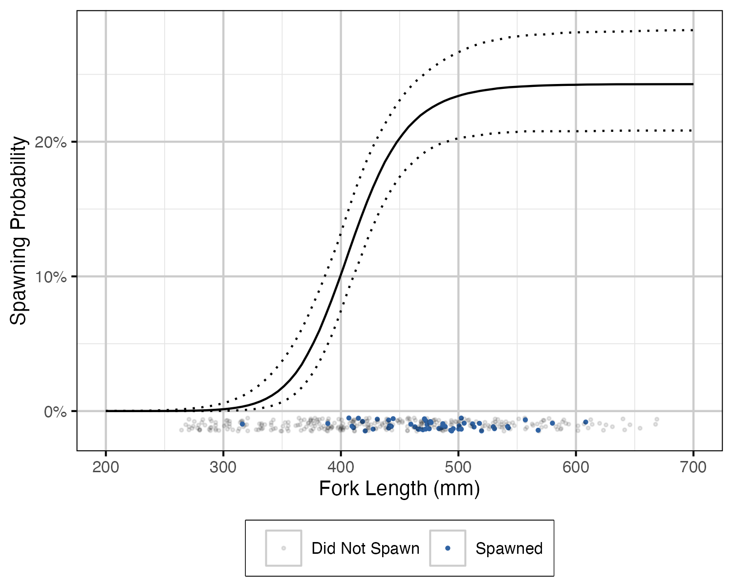
Figure 8. The probability of spawning by fork length (mm) (with 95% CIs). Points represent whether a fish spawned at each spawning opportunity (i.e., spawning period and monitored).
Recommendations
- Data collection
- If feasible, leave receivers in spawning tributaries year-round to observe how often fish are entering outside of the assumed spawning window.
- Analyses
- Add seasonal variation to growth model.
- Estimate effect of study year on spawning probability.
- Estimate effect of study year on recapture probability.
- Estimate effect of fork length on natural mortality using a mechanistic relationship.
Acknowledgements
The organisations and individuals whose contributions have made this analytic appendix possible include:
- Kintama Research Services
- David Welch
- Aswea Porter
- Paul Winchell
- DFO
- Erin Rechisky
- MFLNRORD
- Brendan Andersen
- Mike McCulloch
- Jennifer Sibbald
- Scott Silvestri
- Jaro Szczot