Calculating Water Quality Thresholds and Indices for British Columbia using R
The wqbc R package calculates water quality thresholds and water quality indices and plots water quality indices spatially and temporally for British Columbia.
The package was written for the B.C. Ministry of Environment by Poisson Consulting. Ministry of Environment staff maintain the package. This vignette was primarily written by Colin Millar.
Introduction
The main function of the wqbc (water quality for British Columbia) package is to calculate the Canadian Council of Ministers of the Environment (CCME) water quality index (WQI) for water bodies in British Columbia, the procedure is set out in the CCME WQI (1.0) User’s Manual [@saffran_canadian_2001].
Water quality indices are calculated using the calc_wqi function.
In addition water quality thresholds can be calculated with calc_limits. In this document, thresholds and limits are used interchangeably to describe environmental benchmarks for safe levels of specific substances.
For the visual display of the calculated water quality indices over
a map of British Columbia, the function plot_map is provided.
The purpose of this document is to provide some background to the calculation of indices, provide worked examples of the calculation of indices and and to show how various summaries of the indices can be displayed visually.
The data used in the examples are from the Fraser River basin (data available here under the Candian Open Government License, and an example taken from the CCME WQI User’s Manual [@saffran_canadian_2001].
The following methods of analyzing water quality are provided:
- Calculation of thresholds for water quality variables
- Calculation of the CCME water quality index
- Methods for visualization of water quality indices
The package is intended to be easy to use and provide a flexible means for the exploration of water quality monitoring data. The document is split into the following sections:
- [The CCME Water Quality Index (1.0)]
- [The CCME Example]
- [Data Format]
- [Water Quality Index Calculation]
- [Visual Display of Indices]
The CCME Water Quality Index (1.0)
Water quality is assessed by the monitoring of a range of parameters, referred to in this document as variables. The majority of water quality variables are concentrations of various chemicals, however, quantities such as water turbidity and pH are also important. Comprehensive water quality monitoring has been undertaken in the Fraser River Basin (BC, Canada) since 1979, and this data is provided in the package, however the tools in this package can be applied to any suitable data set provided it meets specific requirements detailed in the [Data Format] section.
The CCME Water Quality Index (1.0) is based on a combination of three factors (F1 to F3):
- F1: Scope the percent of variables where thresholds are exceeded at least once,
- F2: Frequency the percent of individual tests in which thresholds are exceeded, and
- F3: Amplitude the amount by which the thresholds are exceeded.
These are combined to produce a single value (between 0 and 100) which is then converted to a ranking of quality (poor, marginal, fair, good, and excellent) intended to describe overall water quality. In the [Water Quality Index Calculation] section you can see examples of the CCME WQI in action.
The (CCME) WQI is used across Canada as a standardized approach to roll-up the status of multiple water quality parameters at a site and communicate the ‘state’ in a simple manner. The WQI focuses on water quality with respect to the health of freshwater aquatic health. The WQI approach is documented on the CCME website, including detailed methods, a list of established national parameter guidelines/thresholds, and a point and click MS Excel Calculator.
The CCME Example
Lets begin with an example to help understand how the wqbc package works in practice. To begin the package is loaded into R using
library(wqbc)
a good example dataset is that tabled in the CCME WQI (1.0) User’s Manual, which uses a simplified data set from the North Saskatchewan River at Devon, Alberta. A table of the data is given below
| Date | DO | pH | TP | TN | FC | As | Pb | Hg | 2,4-D | Lindane | |
|---|---|---|---|---|---|---|---|---|---|---|---|
| 1 | 1997-01-07 | 11.40 | 8.00 | 0.01 | 0.16 | 4.00 | 0.00 | 0.00 | 0.00 | 0.00 | 0.00 |
| 2 | 1997-02-04 | 11.00 | 7.90 | 0.01 | 0.17 | 0.00 | 0.00 | 0.01 | 0.00 | ||
| 3 | 1997-03-04 | 11.50 | 7.90 | 0.01 | 0.13 | 4.00 | 0.00 | 0.00 | 0.00 | ||
| 4 | 1997-04-08 | 12.50 | 7.90 | 0.06 | 0.43 | 0.00 | 0.00 | 0.00 | 0.00 | 0.00 | 0.00 |
| 5 | 1997-05-06 | 10.40 | 8.10 | 0.04 | 0.25 | 0.00 | 0.00 | 0.00 | 0.00 | ||
| 6 | 1997-06-03 | 8.90 | 8.20 | 0.11 | 0.71 | 26.00 | 0.00 | 0.00 | 0.00 | ||
| 7 | 1997-07-08 | 8.50 | 8.30 | 0.02 | 0.15 | 9.00 | 0.00 | 0.00 | |||
| 8 | 1997-08-05 | 7.50 | 8.20 | 0.01 | 0.15 | 8.00 | 0.00 | 0.00 | 0.00 | 0.00 | 0.00 |
| 9 | 1997-09-02 | 9.20 | 8.20 | 0.01 | 0.13 | 12.00 | 0.00 | 0.00 | 0.00 | ||
| 10 | 1997-10-07 | 11.00 | 8.10 | 0.01 | 0.09 | 12.00 | 0.00 | 0.00 | 0.00 | 0.00 | 0.00 |
| 11 | 1997-11-04 | 12.10 | 8.00 | 0.01 | 0.30 | 8.00 | 0.00 | 0.01 | 0.00 | ||
| 12 | 1997-12-01 | 13.30 | 8.00 | 0.00 | 0.05 | 4.00 | 0.00 | 0.00 | 0.00 |
This data is shipped with the wqbc package and has been called ccme. To load the ccme data into the R session run
data(ccme)
The first 12 rows of the data contain all the data for Dissolved Oxygen (DO) as shown here
head(ccme, 12)
#>          Date Variable Value DetectionLimit LowerLimit UpperLimit Units
#> 1  1997-01-07       DO  11.4             NA          5         NA  Mg/L
#> 2  1997-02-04       DO  11.0             NA          5         NA  Mg/L
#> 3  1997-03-04       DO  11.5             NA          5         NA  Mg/L
#> 4  1997-04-08       DO  12.5             NA          5         NA  Mg/L
#> 5  1997-05-06       DO  10.4             NA          5         NA  Mg/L
#> 6  1997-06-03       DO   8.9             NA          5         NA  Mg/L
#> 7  1997-07-08       DO   8.5             NA          5         NA  Mg/L
#> 8  1997-08-05       DO   7.5             NA          5         NA  Mg/L
#> 9  1997-09-02       DO   9.2             NA          5         NA  Mg/L
#> 10 1997-10-07       DO  11.0             NA          5         NA  Mg/L
#> 11 1997-11-04       DO  12.1             NA          5         NA  Mg/L
#> 12 1997-12-01       DO  13.3             NA          5         NA  Mg/L
Not only are the observed water chemistry values, there is auxiliary information on the analysis methods used, i.e. the detection limits, as well as the lower and upper limits and the units of measurement. The water quality index based on all this data is calculated using the command
calc_wqi(ccme)
#>      WQI Lower Upper Category Variables Tests F1  F2  F3
#> WQI 88.1  87.3  94.2     Good        10   103 20 3.9 2.8
Giving the result 88.1, and given the categories defined in the CCME WQI this equates to a score of ‘Good’. The calc_wqi function gives some additional information. The values for each component of the index are given, so, F1 = 20, F2 = 3.9, and F3 = 2.8. We are also told that there were 10 variables included in the index, which allows us to interpret F1=20 as there being 2 variables which did not meet objectives, however, the proportion of tests not meeting objectives (F2) and the excursions were small (F3) so that these failures are not considered to be a concern. In order to assess the certainty of the classification, confidence intervals are provided for the overall WQI. In this case, both confidence intervals lie within the definition of ‘Good’.
Data Format
There are two datasets provided with the package which follow the data format required by the index calculation routines:
-
[ccme] This dataset contains the CCME (Canadian Council of Ministers of the Environment) Water Quality Index 1.0 User’s Manual example dataset [@saffran_canadian_2001]. The data is a time series of water chemistry measurements taken from North Saskatchewan river at Devon throughout 1997.
-
[Fraser] This dataset contains long term surface freshwater quality monitoring data from the Fraser River Basin (the data was extracted from here where it is provided under the Candian Open Government License) carried out under the Canada-British Columbia Water Quality Monitoring Agreement. Water quality monitoring is conducted to assess water quality status and long-term trends, detect emerging issues, establish water quality guidelines and track the effectiveness of remedial measures and regulatory decisions
The minimal data format is a data frame with columns named, Variable, Value and Units:
#>   Variable Value Units
#> 1       DO  11.4  Mg/L
#> 2       DO  11.0  Mg/L
#> 3       DO  11.5  Mg/L
#> 4       DO  12.5  Mg/L
#> 5       DO  10.4  Mg/L
however, this data can only be used if there are water quality limits defined. The list of variables for which limits are defined can be found using the lookup_limits function
lookup_limits()
#>                         Variable UpperLimit Units
#> 1            Aluminium Dissolved         NA  mg/L
#> 2                  Arsenic Total      5.000  ug/L
#> 3                          Boron      1.200  mg/L
#> 4              Cadmium Dissolved         NA  ug/L
#> 5                 Chloride Total         NA  mg/L
#> 6        Chlorine Total Residual      2.000  ug/L
#> 7                   Cobalt Total      4.000  ug/L
#> 8                   Copper Total         NA  ug/L
#> 9  Cyanide Weak Acid Dissociable      5.000  ug/L
#> 10          Ethinylestradiol 17a      0.500  ng/L
#> 11                  Ethylbenzene      0.200  mg/L
#> 12                          Lead         NA  ug/L
#> 13                     Manganese         NA  mg/L
#> 14                 Mercury Total         NA  ug/L
#> 15   Methyl Tertiary Butyl Ether      3.400  mg/L
#> 16              Molybdenum Total      1.000  mg/L
#> 17                 Nitrate Total      3.000  mg/L
#> 18                       Nitrite         NA  mg/L
#> 19                Selenium Total      0.002  mg/L
#> 20                        Silver         NA  ug/L
#> 21                      Sulphate         NA  mg/L
#> 22                       Toluene      0.039  mg/L
#> 23                    Zinc Total         NA  ug/L
This function will be discussed further in the following section, but note for now that the variable listed as DO (Dissolved Oxygen) in the ccme data does not have a corresponding limit defined in lookup_limits and so for water quality indices to be calculated for the ccme data, there must be thresholds provided for each observation. This should be included by providing
upper limits in a column called UpperLimit, and optionally
lower limits in LowerLimit, for example
head(ccme, 5)
#>         Date Variable Value DetectionLimit LowerLimit UpperLimit Units
#> 1 1997-01-07       DO  11.4             NA          5         NA  Mg/L
#> 2 1997-02-04       DO  11.0             NA          5         NA  Mg/L
#> 3 1997-03-04       DO  11.5             NA          5         NA  Mg/L
#> 4 1997-04-08       DO  12.5             NA          5         NA  Mg/L
#> 5 1997-05-06       DO  10.4             NA          5         NA  Mg/L
To show this in action, lets arbitrarily set all the upper limits in the ccme data to 50, and see what the water quality index is
ccme2 <- ccme
ccme2 $ UpperLimit <- 50
calc_wqi(ccme2)
#> Calculating water quality indices...
#> Deleted 17 rows with missing or negative values in Value.
#> Replaced 31 of the values in column Value with the detection limit in column DetectionLimit.
#> Calculated water quality indices.
#>     WQI Lower Upper  Category Variables Tests F1 F2 F3
#> WQI 100   100   100 Excellent        10   103  0  0  0
And as expected by setting the thresholds arbitrarily high, we get no failures and an Excellent marking!
Water Quality Index Calculation
To explore the functions in more detail a larger data set than ccme is required. Contained in the wqbc package is a second dataset: a copy of the Fraser Basin long term surface freshwater quality monitoring data. To load this data run
data(fraser)
As with the ccme data, the fraser data is organized so that each row corresponds to one observation. The first 10 observations in the fraser dataset are:
head(fraser, 10)
#>        SiteID       Date               Variable   Value Units
#> 1  BC08MB0007 2004-11-15 ALKALINITY TOTAL CACO3  36.900  MG/L
#> 2  BC08MB0007 2004-11-15   ALUMINUM EXTRACTABLE 736.000  UG/L
#> 3  BC08MB0007 2004-11-15         ALUMINUM TOTAL 747.000  UG/L
#> 4  BC08MB0007 2004-11-15      AMMONIA DISSOLVED   0.005  MG/L
#> 5  BC08MB0007 2004-11-15   ANTIMONY EXTRACTABLE   0.044  UG/L
#> 6  BC08MB0007 2004-11-15         ANTIMONY TOTAL   0.045  UG/L
#> 7  BC08MB0007 2004-11-15    ARSENIC EXTRACTABLE   0.430  UG/L
#> 8  BC08MB0007 2004-11-15          ARSENIC TOTAL   0.460  UG/L
#> 9  BC08MB0007 2004-11-15     BARIUM EXTRACTABLE  14.300  UG/L
#> 10 BC08MB0007 2004-11-15           BARIUM TOTAL  14.400  UG/L
#>                                                Site      Lat      Long
#> 1  Chilcotin River upstream of Christie Road Bridge 52.07197 -123.2614
#> 2  Chilcotin River upstream of Christie Road Bridge 52.07197 -123.2614
#> 3  Chilcotin River upstream of Christie Road Bridge 52.07197 -123.2614
#> 4  Chilcotin River upstream of Christie Road Bridge 52.07197 -123.2614
#> 5  Chilcotin River upstream of Christie Road Bridge 52.07197 -123.2614
#> 6  Chilcotin River upstream of Christie Road Bridge 52.07197 -123.2614
#> 7  Chilcotin River upstream of Christie Road Bridge 52.07197 -123.2614
#> 8  Chilcotin River upstream of Christie Road Bridge 52.07197 -123.2614
#> 9  Chilcotin River upstream of Christie Road Bridge 52.07197 -123.2614
#> 10 Chilcotin River upstream of Christie Road Bridge 52.07197 -123.2614
In this dataset the auxiliary data available are a site identifier (SiteID), the site name in full (Site), and the position in terms of latitude (Lat) and longitude (Long). This information can be used to visualize the site positions on a map, and through the use of coloured symbols, additional information, such as the site name, can be included.
plot_map(fraser, fill = "SiteID")
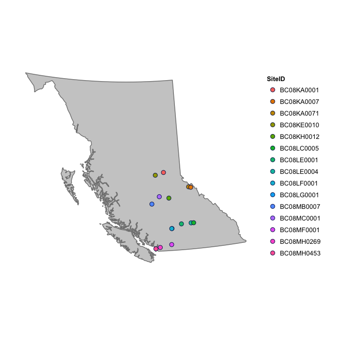
For more information on plotting see the section on [Visual Display of Indices]. This will be particularly useful when summarizing the results of the water quality index calculations.
To calculate the long-term water quality index for each site all that needs to be done is to run
calc_wqi(fraser, by = "SiteID")
But this does not help to explain what is going on which is the purpose of this section.
cleaning and standardising data
The fraser data is a large dataset, and to get things started we will use a subset of this data. Lets take the data from 2012. A useful package for working with the dates is the lubridate package. We will use the function year from the lubridate package to help subset the data. Before using the year function you should make sure the lubridate package is loaded by running library(lubridate).
library(lubridate)
data2012 <- subset(fraser, year(Date) == 2012)
head(data2012)
#>           SiteID       Date               Variable    Value Units
#> 12659 BC08MB0007 2012-01-10 ALKALINITY TOTAL CACO3  55.2000  MG/L
#> 12660 BC08MB0007 2012-01-10         ALUMINUM TOTAL 318.0000  UG/L
#> 12661 BC08MB0007 2012-01-10      AMMONIA DISSOLVED   0.0103  MG/L
#> 12662 BC08MB0007 2012-01-10         ANTIMONY TOTAL   0.0470  UG/L
#> 12663 BC08MB0007 2012-01-10          ARSENIC TOTAL   0.4600  UG/L
#> 12664 BC08MB0007 2012-01-10           BARIUM TOTAL  11.2000  UG/L
#>                                                   Site      Lat      Long
#> 12659 Chilcotin River upstream of Christie Road Bridge 52.07197 -123.2614
#> 12660 Chilcotin River upstream of Christie Road Bridge 52.07197 -123.2614
#> 12661 Chilcotin River upstream of Christie Road Bridge 52.07197 -123.2614
#> 12662 Chilcotin River upstream of Christie Road Bridge 52.07197 -123.2614
#> 12663 Chilcotin River upstream of Christie Road Bridge 52.07197 -123.2614
#> 12664 Chilcotin River upstream of Christie Road Bridge 52.07197 -123.2614
We are now in a position to calculate the long term water quality index for 2012, and as previously stated, this is done using
calc_wqi(data2012)
The function calc_wqi performs a number of tasks. The first of these is to check if the dataset contains user defined limits in columns called UpperLimit or LowerLimit. If the dataset has these columns, the function proceeds directly to calculating the water quality index.
If the data do not contain user defined limits, as is the case for the fraser dataset, the next steps are to check and standardize the data so that they can be matched with known water quality limits. The list of known water quality limits can be queried using the function lookup_limits, which has arguments to help evaluate the limit. Because some limits are dependent on the concentrations of other chemicals, lookup_limits has the following arguments: ph, hardness, chloride and methyl_mercury. In addition because limits are different depending on the time scale, there is a further argument term which can take the values “short” or “long” (defined later in [Calculating limits]).
lookup_limits(ph = 7)
#>                         Variable UpperLimit Units
#> 1            Aluminium Dissolved      0.050  mg/L
#> 2                  Arsenic Total      5.000  ug/L
#> 3                          Boron      1.200  mg/L
#> 4              Cadmium Dissolved         NA  ug/L
#> 5                 Chloride Total         NA  mg/L
#> 6        Chlorine Total Residual      2.000  ug/L
#> 7                   Cobalt Total      4.000  ug/L
#> 8                   Copper Total         NA  ug/L
#> 9  Cyanide Weak Acid Dissociable      5.000  ug/L
#> 10          Ethinylestradiol 17a      0.500  ng/L
#> 11                  Ethylbenzene      0.200  mg/L
#> 12                          Lead         NA  ug/L
#> 13                     Manganese         NA  mg/L
#> 14                 Mercury Total         NA  ug/L
#> 15   Methyl Tertiary Butyl Ether      3.400  mg/L
#> 16              Molybdenum Total      1.000  mg/L
#> 17                 Nitrate Total      3.000  mg/L
#> 18                       Nitrite         NA  mg/L
#> 19                Selenium Total      0.002  mg/L
#> 20                        Silver         NA  ug/L
#> 21                      Sulphate         NA  mg/L
#> 22                       Toluene      0.039  mg/L
#> 23                    Zinc Total         NA  ug/L
From this we can see that there are 23 standard variables with limits defined. Some variable in the previous example have NA because these limits require knowledge of hardness, chloride or methyl mercury concentrations.
The first step in assigning these limits to observations involves converting any non-standard variable names, checking and converting the units, and removing any missing and negative values. Although this is done within the calc_wqi function, it can be useful to run a manual check on the data first. This is done using the standardize_wqdata function
data2012 <- standardize_wqdata(data2012)
#> Standardizing water quality data...
#> Deleted 45 rows with negative values in Value.
#> Substituted 'ALUMINUM DISSOLVED' with 'Aluminium Dissolved', 'ARSENIC TOTAL' with 'Arsenic Total', 'BORON DISSOLVED' with 'Boron', 'BORON TOTAL' with 'Boron', 'CADMIUM DISSOLVED' with 'Cadmium Dissolved', 'COBALT TOTAL' with 'Cobalt Total', 'COPPER TOTAL' with 'Copper Total', 'CYANIDE WEAK ACID DISSOCIABLE' with 'Cyanide Weak Acid Dissociable', 'HARDNESS TOTAL (CALCD.) CACO3' with 'Hardness Total', 'IRON DISSOLVED' with 'Iron Dissolved', 'IRON TOTAL' with 'Iron Total', 'LEAD DISSOLVED' with 'Lead', 'LEAD TOTAL' with 'Lead', 'MANGANESE DISSOLVED' with 'Manganese', 'MANGANESE TOTAL' with 'Manganese', 'MOLYBDENUM TOTAL' with 'Molybdenum Total', 'NITROGEN NITRITE' with 'Nitrite', 'PH' with 'pH', 'PH - FIELD' with 'pH', 'SELENIUM TOTAL' with 'Selenium Total', 'SILVER DISSOLVED' with 'Silver', 'SILVER TOTAL' with 'Silver', 'SULPHATE DISSOLVED' with 'Sulphate' and 'ZINC TOTAL' with 'Zinc Total'.
#> Failed to substitute 'ALKALINITY GRAN CACO3', 'ALKALINITY TOTAL CACO3', 'ALUMINUM TOTAL', 'AMMONIA DISSOLVED', 'ANTIMONY DISSOLVED', 'ANTIMONY TOTAL', 'ARSENIC DISSOLVED', 'BARIUM DISSOLVED', 'BARIUM TOTAL', 'BERYLLIUM DISSOLVED', 'BERYLLIUM TOTAL', 'BISMUTH DISSOLVED', 'BISMUTH TOTAL', 'CADMIUM TOTAL', 'CALCIUM DISSOLVED', 'CALCIUM TOTAL', 'CARBON DISSOLVED INORGANIC', 'CARBON DISSOLVED ORGANIC', 'CARBON TOTAL INORGANIC', 'CARBON TOTAL ORGANIC', 'CERIUM DISSOLVED', 'CERIUM TOTAL', 'CESIUM DISSOLVED', 'CESIUM TOTAL', 'CHLORIDE DISSOLVED', 'CHROMIUM DISSOLVED', 'CHROMIUM TOTAL', 'COBALT DISSOLVED', 'COLIFORMS FECAL', 'COLOUR TRUE', 'COPPER DISSOLVED', 'CYANIDE TOTAL', 'ENTEROCOCUS', 'ESCHERICHIA COLI', 'FLUORIDE DISSOLVED', 'GALLIUM DISSOLVED', 'GALLIUM TOTAL', 'LANTHANUM DISSOLVED', 'LANTHANUM TOTAL', 'LITHIUM DISSOLVED', 'LITHIUM TOTAL', 'MAGNESIUM DISSOLVED', 'MAGNESIUM TOTAL', 'MOLYBDENUM DISSOLVED', 'NICKEL DISSOLVED', 'NICKEL TOTAL', 'NIOBIUM DISSOLVED', 'NIOBIUM TOTAL', 'NITROGEN DISSOLVED KJELDAHL', 'NITROGEN DISSOLVED NITRATE', 'NITROGEN DISSOLVED NO3 & NO2', 'NITROGEN DISSOLVED ORGANIC (CALCD.)', 'NITROGEN TOTAL', 'NITROGEN TOTAL DISSOLVED', 'NITROGEN TOTAL KJELDAHL', 'NITROGEN TOTAL ORGANIC (CALCD.)', 'OXYGEN DISSOLVED', 'PHOSPHORUS DISSOLVED ORTHO', 'PHOSPHORUS TOTAL', 'PHOSPHORUS TOTAL DISSOLVED', 'PLATINUM DISSOLVED', 'PLATINUM TOTAL', 'POTASSIUM DISSOLVED', 'POTASSIUM TOTAL', 'RESIDUE FILTERABLE', 'RESIDUE NONFILTRABLE', 'RESIDUE TOTAL', 'RUBIDIUM DISSOLVED', 'RUBIDIUM TOTAL', 'SALINITY', 'SELENIUM DISSOLVED', 'SILICON DISSOLVED', 'SILICON TOTAL', 'SODIUM DISSOLVED', 'SODIUM TOTAL', 'SPECIFIC CONDUCTANCE', 'SPECIFIC CONDUCTANCE - FIELD', 'STRONTIUM DISSOLVED', 'STRONTIUM TOTAL', 'SULPHUR DISSOLVED', 'SULPHUR TOTAL', 'TEMPERATURE AIR', 'TEMPERATURE WATER', 'THALLIUM DISSOLVED', 'THALLIUM TOTAL', 'TIN DISSOLVED', 'TIN TOTAL', 'TITANIUM DISSOLVED', 'TITANIUM TOTAL', 'TUNGSTEN DISSOLVED', 'TUNGSTEN TOTAL', 'TURBIDITY', 'URANIUM DISSOLVED', 'URANIUM TOTAL', 'VANADIUM DISSOLVED', 'VANADIUM TOTAL', 'YTTRIUM DISSOLVED', 'YTTRIUM TOTAL', 'ZINC DISSOLVED', 'ZIRCONIUM DISSOLVED' and 'ZIRCONIUM TOTAL'.
#> Deleted 13823 rows with missing values in Variable.
#> Substituted 'MG/L' with 'mg/L', 'PH UNITS' with 'pH' and 'UG/L' with 'ug/L'.
#> Standardized water quality data.
head(data2012)
#>       SiteID       Date            Variable  Value Units
#> 1 BC08MH0453 2012-04-13 Aluminium Dissolved 0.0511  mg/L
#> 2 BC08MH0453 2012-05-16 Aluminium Dissolved 0.0043  mg/L
#> 3 BC08MH0453 2012-06-21 Aluminium Dissolved 0.1320  mg/L
#> 4 BC08MH0453 2012-06-21 Aluminium Dissolved 0.1390  mg/L
#> 5 BC08MH0453 2012-06-21 Aluminium Dissolved 0.1310  mg/L
#> 6 BC08MH0453 2012-07-13 Aluminium Dissolved 0.0664  mg/L
#>                                                Site    Lat     Long
#> 1 Fraser River (Main Arm) at Gravesend Reach - Buoy 49.167 -123.035
#> 2 Fraser River (Main Arm) at Gravesend Reach - Buoy 49.167 -123.035
#> 3 Fraser River (Main Arm) at Gravesend Reach - Buoy 49.167 -123.035
#> 4 Fraser River (Main Arm) at Gravesend Reach - Buoy 49.167 -123.035
#> 5 Fraser River (Main Arm) at Gravesend Reach - Buoy 49.167 -123.035
#> 6 Fraser River (Main Arm) at Gravesend Reach - Buoy 49.167 -123.035
Note that the effect of running standardize_wqdata is to convert some variable names to a standard form, for example, ‘ALUMINUM DISSOLVED’ has been replaced with ‘Aluminium Dissolved’. The messages output by the function relay this information, along with all the other substitutions made. In addition, there are a number of variable names which are not part of the standard list of variables and were removed from the dataset. Unit names are also standardized, for example ‘MG/L’ has been replaced with ‘mg/L’, there are also some unrecognized units which result in the related observations being removed from the dataset. As a result of the standardization, the 2012 Fraser dataset has been reduced from 18062 recorded observations, to 4194 standard observations, which can all be matched with the thresholds.
After standardization, it is necessary to ensure that there are only single values for each date for a given variable and this is done using the function clean_wqdata. If the data is to be considered as observations of one entity, i.e. the whole Fraser river basin, then this function will average over all data occurring on a given day. If this was desired, the following code would be used
clean_wqdata(data2012)
However, with the Fraser river basin data it makes more sense to consider the data as observations of different sites within the river basin. To tell the clean_wqdata function to average observations within site, the argument by is used
data2012 <- clean_wqdata(data2012, by = "SiteID")
#> Standardizing water quality data...
#> Standardized water quality data.
#> Cleaning water quality data...
#> Cleansed water quality data.
In this case there are no problems, and the data is ready for the next step. Note that, to be on the safe side, the function clean_wqdata runs a standardization again, in case it wasn’t done previously.
Calculating limits
Now that we have observations for a range of standard variables it is possible to calculate the relevant limits with which to assess exceedances. Taking into account the various rules for calculating thresholds for the standard variables, the function calc_limits calculates the limits required to evaluate the water quality index. Again, if it is required to calculate the water quality index for each site, then the by argument is used
calc_limits(data2012, by = "SiteID", term = "long")
#> Standardizing water quality data...
#> Standardized water quality data.
#> Cleaning water quality data...
#> Cleansed water quality data.
#> Calculating long-term water quality limits...
#> Calculated long-term water quality limits.
#>        SiteID       Date         Variable      Value UpperLimit Units
#> 1  BC08MC0001 2012-04-11    Arsenic Total  1.8500000   5.000000  ug/L
#> 2  BC08MC0001 2012-04-11            Boron  0.0024400   1.200000  mg/L
#> 3  BC08MC0001 2012-04-11     Cobalt Total  4.5840000   4.000000  ug/L
#> 4  BC08MC0001 2012-04-11     Copper Total 13.8340000   2.332800  ug/L
#> 5  BC08MC0001 2012-04-11             Lead  3.0680000   4.913114  ug/L
#> 6  BC08MC0001 2012-04-11        Manganese  0.2528000   0.861608  mg/L
#> 7  BC08MC0001 2012-04-11 Molybdenum Total  0.0005056   1.000000  mg/L
#> 8  BC08MC0001 2012-04-11   Selenium Total  0.0001440   0.002000  mg/L
#> 9  BC08MC0001 2012-04-11           Silver  0.0538000   0.050000  ug/L
#> 10 BC08MC0001 2012-04-11       Zinc Total 23.4400000   7.500000  ug/L
Now the 2012 Fraser River basin data has been reduced to daily means of the standard variables, and thresholds have been attributed to each observation. A visual inspection of the data shows that for the period starting the 11th April, several variables at the BC08MC0001 site are above their long-term limits, i.e. Cobalt Total, Copper Total, Silver and Zinc Total.
Long or Short term
In the previous output, the calc_limits function returned a total of ten limits, all with the same date and all from the same site. But what is going on? A plot of the 2012 data show that there are observations throughout the year from a number of different sites. (Note this plot requires the use of the library ggplot2, which is loaded using library(ggplot2))
qplot(Date, SiteID, xlab = "", ylab = "", data = data2012, colour = SiteID == "BC08MC0001")
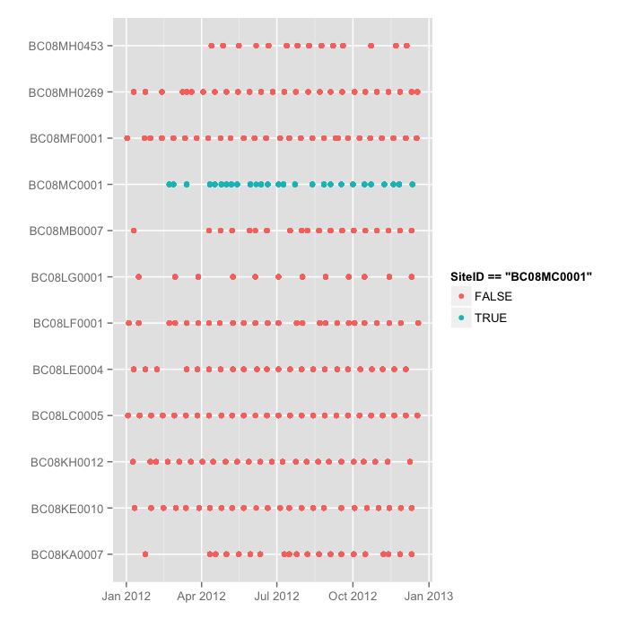
The point here is that the calc_limits function can calculate long or short-term limits. For long-term limits, thresholds are calculated for each 30 day period. Then in the water quality calculation, these 30 day periods are treated as individual test units for exceedances. There are strict rules applied to whether a 30 day period is considered valid for limit calculation: there must be at least 5 values spanning at least 21 days in a 30 day period for that period to be valid, and since replicates are averaged (by the clean_wqdata function) prior to calculating the limits each of the 5 values must occur on a separate date. This explains why the long term limits, by site are so few for the 2012 data: only the BC08MC0001 site has sufficiently frequent observations, occurring once in the year in the 30 day period following the 11th of April, to be considered valid for the calculation of long-term limits.
The strict conditions required for long-term limits are not required when calculating short-term limits, where instead individual days are considered as the test units for exceedances.
data2012 <- calc_limits(data2012, by = "SiteID", term = "short")
#> Standardizing water quality data...
#> Standardized water quality data.
#> Cleaning water quality data...
#> Cleansed water quality data.
#> Calculating short-term water quality limits...
#> Calculated short-term water quality limits.
head(data2012, 12)
#>        SiteID       Date         Variable   Value UpperLimit Units
#> 1  BC08KA0007 2012-01-24     Cobalt Total 0.20000 110.000000  ug/L
#> 2  BC08KA0007 2012-01-24     Copper Total 0.45000   9.491800  ug/L
#> 3  BC08KA0007 2012-01-24       Iron Total 0.03030   1.000000  mg/L
#> 4  BC08KA0007 2012-01-24             Lead 0.01000  61.162679  ug/L
#> 5  BC08KA0007 2012-01-24        Manganese 0.01120   1.418294  mg/L
#> 6  BC08KA0007 2012-01-24 Molybdenum Total 0.00007   2.000000  mg/L
#> 7  BC08KA0007 2012-01-24           Silver 0.00100   0.100000  ug/L
#> 8  BC08KA0007 2012-01-24       Zinc Total 0.30000  33.000000  ug/L
#> 9  BC08KA0007 2012-04-11     Cobalt Total 0.20000 110.000000  ug/L
#> 10 BC08KA0007 2012-04-11     Copper Total 0.42000   9.679800  ug/L
#> 11 BC08KA0007 2012-04-11       Iron Total 0.04450   1.000000  mg/L
#> 12 BC08KA0007 2012-04-11             Lead 0.02100  63.123160  ug/L
Calculating the Water Quality Index
Note that the default for calculating the water quality index is the use of long-term limits, but for the sake of continuing the example, we will keep with the 2012 data. Lets begin by summarizing the steps so far: The full Fraser river basin dataset was subset to retain only the data from 2012. Then this data (which we have called data2012) was first, standardized, cleaned and then the limits were calculated for daily values.
data2012 <- subset(fraser, year(Date) == 2012)
data2012 <- standardize_wqdata(data2012)
data2012 <- clean_wqdata(data2012, by = "SiteID")
data2012 <- calc_limits(data2012, by = "SiteID", term = "short")
The data is now ready to have the water quality index calculated for each site, and this is done using
wqi2012 <- calc_wqi(data2012, by = "SiteID")
#> Calculating water quality indices...
#> Added missing column LowerLimit to x.
#> Added missing column DetectionLimit to x.
#> Calculated water quality indices.
wqi2012
#>        SiteID   WQI Lower Upper  Category Variables Tests   F1   F2   F3
#> 1  BC08KA0007 100.0 100.0 100.0 Excellent         8   160  0.0  0.0  0.0
#> 2  BC08KE0010  92.7  92.3 100.0      Good         8   184 12.5  1.1  1.4
#> 3  BC08KH0012  89.5  85.4 100.0      Good        11   195 18.2  1.0  0.7
#> 4  BC08LC0005  93.6  93.5 100.0      Good         9   226 11.1  0.4  0.0
#> 5  BC08LE0004  86.8  85.9  93.5      Good         9   204 22.2  3.4  4.0
#> 6  BC08LF0001  85.5  85.2 100.0      Good         8   200 25.0  2.0  1.4
#> 7  BC08LG0001  85.2  83.8 100.0      Good         8    96 25.0  3.1  4.3
#> 8  BC08MB0007  85.0  83.4  92.6      Good         8   144 25.0  5.6  4.8
#> 9  BC08MC0001  73.1  68.9  82.9      Fair         8   208 37.5 12.0 24.8
#> 10 BC08MF0001  82.8  80.2  84.7      Good         8   216 25.0  9.3 13.4
#> 11 BC08MH0269 100.0 100.0 100.0 Excellent        10   212  0.0  0.0  0.0
#> 12 BC08MH0453  83.2  80.8  94.2      Good        11   140 27.3  7.9  6.8
Due to the sampling frequency in 2012, it is not possible to calculate long term limits, because there are not enough samples in each 30 day period for each site. A long-term water quality index for 2012 can be calculated for the whole river basin:
data2012 <- subset(fraser, year(Date) == 2012)
calc_wqi(data2012)
#>     WQI Lower Upper Category Variables Tests   F1  F2  F3
#> WQI  90  88.3  95.1     Good        12   121 16.7 4.1 2.5
Visual Display of Indices
In order to display the indices, it is required to retain the spatial location of the sites through the analysis. This can be done by amending the code used previously to calculate WQI for 2012. We will take a short cut this time and use the fact that calc_limits standardizes and cleans the data before calculating limits. One way to keep the latitude and longitude information is to add it to the by argument. Because each siteID always has the same latitude and longitude, the effect of this will be to have additional columns in the output from calc_limits. We can also turn off messages about variable name substitution if desired
options(wqbc.messages = FALSE)
data2012 <- subset(fraser, year(Date) == 2012)
data2012 <- calc_limits(data2012, by = c("SiteID", "Lat", "Long"), term = "short")
head(data2012)
#>       SiteID     Lat      Long       Date         Variable   Value
#> 1 BC08KA0007 52.9878 -119.0101 2012-01-24     Cobalt Total 0.20000
#> 2 BC08KA0007 52.9878 -119.0101 2012-01-24     Copper Total 0.45000
#> 3 BC08KA0007 52.9878 -119.0101 2012-01-24       Iron Total 0.03030
#> 4 BC08KA0007 52.9878 -119.0101 2012-01-24             Lead 0.01000
#> 5 BC08KA0007 52.9878 -119.0101 2012-01-24        Manganese 0.01120
#> 6 BC08KA0007 52.9878 -119.0101 2012-01-24 Molybdenum Total 0.00007
#>   UpperLimit Units
#> 1 110.000000  ug/L
#> 2   9.491800  ug/L
#> 3   1.000000  mg/L
#> 4  61.162679  ug/L
#> 5   1.418294  mg/L
#> 6   2.000000  mg/L
Now when the water quality index is calculated, we have to pass the additional columns again to retain latitude and longitude in the output from calc_wqi
wqi2012 <- calc_wqi(data2012, by = c("SiteID", "Lat", "Long"))
wqi2012
#>        SiteID      Lat      Long   WQI Lower Upper  Category Variables
#> 1  BC08KA0007 52.98780 -119.0101 100.0 100.0 100.0 Excellent         8
#> 2  BC08KE0010 53.92722 -122.7650  92.7  92.3 100.0      Good         8
#> 3  BC08KH0012 52.40330 -121.4342  89.5  85.5 100.0      Good        11
#> 4  BC08LC0005 50.68484 -119.0700  93.6  93.5 100.0      Good         9
#> 5  BC08LE0004 50.69139 -119.3289  86.8  85.8  93.5      Good         9
#> 6  BC08LF0001 50.42083 -121.3414  85.5  85.2 100.0      Good         8
#> 7  BC08LG0001 50.42500 -121.3164  85.2  83.8 100.0      Good         8
#> 8  BC08MB0007 52.07197 -123.2614  85.0  83.5  92.6      Good         8
#> 9  BC08MC0001 52.52964 -122.4423  73.1  68.7  83.0      Fair         8
#> 10 BC08MF0001 49.38722 -121.4508  82.8  80.3  84.7      Good         8
#> 11 BC08MH0269 49.24211 -122.5961 100.0 100.0 100.0 Excellent        10
#> 12 BC08MH0453 49.16700 -123.0350  83.2  81.1  89.4      Good        11
#>    Tests   F1   F2   F3
#> 1    160  0.0  0.0  0.0
#> 2    184 12.5  1.1  1.4
#> 3    195 18.2  1.0  0.7
#> 4    226 11.1  0.4  0.0
#> 5    204 22.2  3.4  4.0
#> 6    200 25.0  2.0  1.4
#> 7     96 25.0  3.1  4.3
#> 8    144 25.0  5.6  4.8
#> 9    208 37.5 12.0 24.8
#> 10   216 25.0  9.3 13.4
#> 11   212  0.0  0.0  0.0
#> 12   140 27.3  7.9  6.8
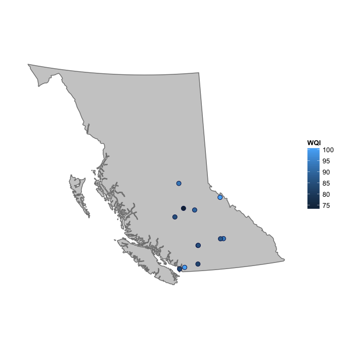
Since this data now has the coordinates of each site, we can plot the index on a map using the function used at the start of the [Water quality index calculation] section.
plot_map(wqi2012, fill = "WQI")
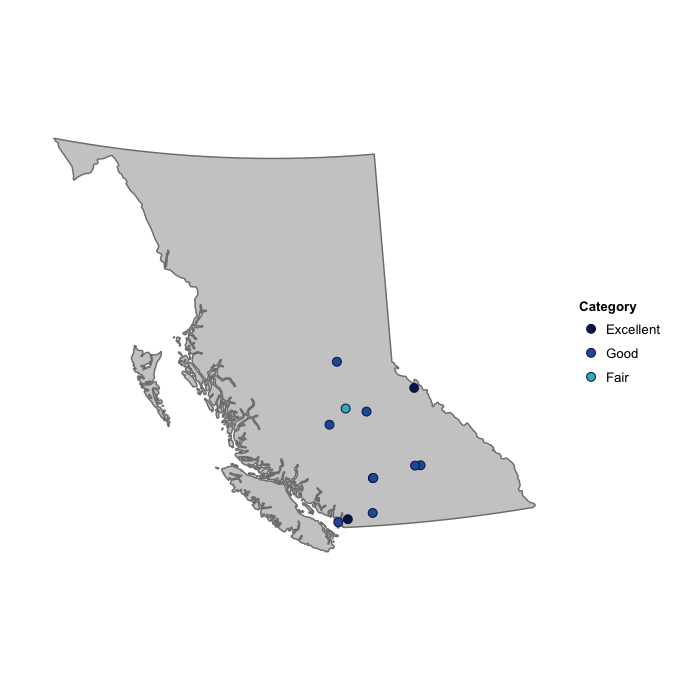
However, there is a special plotting function designed especially for plotting the results of calc_wqi, and this is plot_map_wqis
plot_map_wqis(wqi2012)
Additional Examples
An example calculating water quality indices for grouped sites
This first example shows how it is possible to create a group of sites, in this case it is based on latitude, the group South is below 52 degrees latitude, while the sites above this line are in the North group. Short term water quality indices for 2012 are calculated for these groups using the following
options(wqbc.messages = FALSE)
dataNorthSouth <- subset(fraser, year(Date) %in% 2012)
dataNorthSouth $ NorthSouth <- ifelse(dataNorthSouth $ Lat < 52, "South", "North")
limitsNorthSouth <- calc_limits(dataNorthSouth, by = "NorthSouth", term = "short")
wqiNorthSouth <- calc_wqi(limitsNorthSouth, by = "NorthSouth")
Then to attribute these grouped water quality indices back to the individual sites, a basic R function called merge is used, which merges based on column names. An additional trick is used here where the function unique keeps only the unique combinations of NorthSouth, SiteID, Lat and Long.
wqiNorthSouth <- merge(unique(dataNorthSouth[c("NorthSouth", "SiteID", "Lat", "Long")]), wqiNorthSouth)
wqiNorthSouth
#>    NorthSouth     SiteID      Lat      Long  WQI Lower Upper Category
#> 1       North BC08MB0007 52.07197 -123.2614 83.5  77.2  89.3     Good
#> 2       North BC08KH0012 52.40330 -121.4342 83.5  77.2  89.3     Good
#> 3       North BC08KE0010 53.92722 -122.7650 83.5  77.2  89.3     Good
#> 4       North BC08MC0001 52.52964 -122.4423 83.5  77.2  89.3     Good
#> 5       North BC08KA0007 52.98780 -119.0101 83.5  77.2  89.3     Good
#> 6       South BC08MH0453 49.16700 -123.0350 85.1  84.7  90.0     Good
#> 7       South BC08MF0001 49.38722 -121.4508 85.1  84.7  90.0     Good
#> 8       South BC08LG0001 50.42500 -121.3164 85.1  84.7  90.0     Good
#> 9       South BC08MH0269 49.24211 -122.5961 85.1  84.7  90.0     Good
#> 10      South BC08LE0004 50.69139 -119.3289 85.1  84.7  90.0     Good
#> 11      South BC08LC0005 50.68484 -119.0700 85.1  84.7  90.0     Good
#> 12      South BC08LF0001 50.42083 -121.3414 85.1  84.7  90.0     Good
#>    Variables Tests   F1  F2  F3
#> 1         11   683 27.3 4.0 7.4
#> 2         11   683 27.3 4.0 7.4
#> 3         11   683 27.3 4.0 7.4
#> 4         11   683 27.3 4.0 7.4
#> 5         11   683 27.3 4.0 7.4
#> 6         12   921 25.0 4.1 4.7
#> 7         12   921 25.0 4.1 4.7
#> 8         12   921 25.0 4.1 4.7
#> 9         12   921 25.0 4.1 4.7
#> 10        12   921 25.0 4.1 4.7
#> 11        12   921 25.0 4.1 4.7
#> 12        12   921 25.0 4.1 4.7
plot_map(wqiNorthSouth, fill = "WQI")

Sites could be grouped based on other attributes if these were available, such as altitude for example.
An example over multiple years
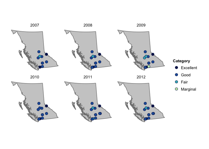
This example calculates short term water quality indices over multiple years (in this case from 2002 to 2012), and by site. The function facet_wrap is then used to produce a gridded plot output showing multiple years
options(wqbc.messages = TRUE)
data07to12 <- subset(fraser, year(Date) %in% 2007:2012)
data07to12 $ year <- year(data07to12 $ Date)
limits07to12 <- calc_limits(data07to12, by = c("year", "SiteID", "Lat", "Long"), term = "short")
#> Standardizing water quality data...
#> Deleted 253 rows with negative values in Value.
#> Substituted 'ALUMINUM DISSOLVED' with 'Aluminium Dissolved', 'ARSENIC TOTAL' with 'Arsenic Total', 'BORON DISSOLVED' with 'Boron', 'BORON EXTRACTABLE' with 'Boron', 'BORON TOTAL' with 'Boron', 'CADMIUM DISSOLVED' with 'Cadmium Dissolved', 'COBALT TOTAL' with 'Cobalt Total', 'COPPER TOTAL' with 'Copper Total', 'CYANIDE WEAK ACID DISSOCIABLE' with 'Cyanide Weak Acid Dissociable', 'HARDNESS TOTAL (CALCD.) CACO3' with 'Hardness Total', 'IRON DISSOLVED' with 'Iron Dissolved', 'IRON TOTAL' with 'Iron Total', 'LEAD DISSOLVED' with 'Lead', 'LEAD EXTRACTABLE' with 'Lead', 'LEAD TOTAL' with 'Lead', 'MANGANESE DISSOLVED' with 'Manganese', 'MANGANESE EXTRACTABLE' with 'Manganese', 'MANGANESE TOTAL' with 'Manganese', 'MOLYBDENUM TOTAL' with 'Molybdenum Total', 'NITROGEN NITRITE' with 'Nitrite', 'PH' with 'pH', 'PH - FIELD' with 'pH', 'SELENIUM TOTAL' with 'Selenium Total', 'SILVER DISSOLVED' with 'Silver', 'SILVER EXTRACTABLE' with 'Silver', 'SILVER TOTAL' with 'Silver', 'SULPHATE DISSOLVED' with 'Sulphate' and 'ZINC TOTAL' with 'Zinc Total'.
#> Failed to substitute 'ADSORBABLE ORGANIC HALIDE - AOX', 'ALKALINITY GRAN CACO3', 'ALKALINITY PHENOLPHTHALEIN CACO3', 'ALKALINITY TOTAL CACO3', 'ALUMINUM EXTRACTABLE', 'ALUMINUM TOTAL', 'ALUMINUM_27 TOTAL RECOVERABLE - AL', 'AMMONIA DISSOLVED', 'ANTIMONY DISSOLVED', 'ANTIMONY EXTRACTABLE', 'ANTIMONY TOTAL', 'ARSENIC DISSOLVED', 'ARSENIC EXTRACTABLE', 'BARIUM DISSOLVED', 'BARIUM EXTRACTABLE', 'BARIUM TOTAL', 'BERYLLIUM DISSOLVED', 'BERYLLIUM EXTRACTABLE', 'BERYLLIUM TOTAL', 'BICARBONATE (CALCD.)', 'BISMUTH DISSOLVED', 'BISMUTH EXTRACTABLE', 'BISMUTH TOTAL', 'BROMIDE DISSOLVED', 'CADMIUM EXTRACTABLE', 'CADMIUM TOTAL', 'CALCIUM DISSOLVED', 'CALCIUM EXTRACTABLE', 'CALCIUM TOTAL', 'CARBON DISSOLVED INORGANIC', 'CARBON DISSOLVED ORGANIC', 'CARBON TOTAL INORGANIC', 'CARBON TOTAL ORGANIC', 'CARBONATE (CALCD.)', 'CERIUM DISSOLVED', 'CERIUM EXTRACTABLE', 'CERIUM TOTAL', 'CESIUM DISSOLVED', 'CESIUM EXTRACTABLE', 'CESIUM TOTAL', 'CHLORIDE DISSOLVED', 'CHROMIUM DISSOLVED', 'CHROMIUM EXTRACTABLE', 'CHROMIUM TOTAL', 'COBALT DISSOLVED', 'COBALT EXTRACTABLE', 'COLIFORMS FECAL', 'COLOUR APPARENT', 'COLOUR TRUE', 'COPPER DISSOLVED', 'COPPER EXTRACTABLE', 'CYANIDE TOTAL', 'ENTEROCOCUS', 'ESCHERICHIA COLI', 'FLUORIDE DISSOLVED', 'GALLIUM DISSOLVED', 'GALLIUM EXTRACTABLE', 'GALLIUM TOTAL', 'HYDROXIDE (CALCD.)', 'IRON EXTRACTABLE', 'LANTHANUM DISSOLVED', 'LANTHANUM EXTRACTABLE', 'LANTHANUM TOTAL', 'LITHIUM DISSOLVED', 'LITHIUM EXTRACTABLE', 'LITHIUM TOTAL', 'MAGNESIUM DISSOLVED', 'MAGNESIUM EXTRACTABLE', 'MAGNESIUM TOTAL', 'MERCURY DISSOLVED', 'MOLYBDENUM DISSOLVED', 'MOLYBDENUM EXTRACTABLE', 'NICKEL DISSOLVED', 'NICKEL EXTRACTABLE', 'NICKEL TOTAL', 'NIOBIUM DISSOLVED', 'NIOBIUM EXTRACTABLE', 'NIOBIUM TOTAL', 'NITROGEN DISSOLVED KJELDAHL', 'NITROGEN DISSOLVED NITRATE', 'NITROGEN DISSOLVED NO3 & NO2', 'NITROGEN DISSOLVED ORGANIC (CALCD.)', 'NITROGEN TOTAL', 'NITROGEN TOTAL DISSOLVED', 'NITROGEN TOTAL KJELDAHL', 'NITROGEN TOTAL ORGANIC (CALCD.)', 'OXYGEN DISSOLVED', 'PHOSPHORUS DISSOLVED ORTHO', 'PHOSPHORUS TOTAL', 'PHOSPHORUS TOTAL DISSOLVED', 'PLATINUM DISSOLVED', 'PLATINUM EXTRACTABLE', 'PLATINUM TOTAL', 'POTASSIUM DISSOLVED', 'POTASSIUM EXTRACTABLE', 'POTASSIUM TOTAL', 'RESIDUE FILTERABLE', 'RESIDUE NONFILTRABLE', 'RESIDUE TOTAL', 'RUBIDIUM DISSOLVED', 'RUBIDIUM EXTRACTABLE', 'RUBIDIUM TOTAL', 'SALINITY', 'SELENIUM DISSOLVED', 'SELENIUM EXTRACTABLE', 'SILICON DISSOLVED', 'SILICON EXTRACTABLE', 'SILICON TOTAL', 'SODIUM DISSOLVED', 'SODIUM EXTRACTABLE', 'SODIUM TOTAL', 'SPECIFIC CONDUCTANCE', 'SPECIFIC CONDUCTANCE - FIELD', 'STRONTIUM DISSOLVED', 'STRONTIUM EXTRACTABLE', 'STRONTIUM TOTAL', 'SULPHUR DISSOLVED', 'SULPHUR TOTAL', 'TEMPERATURE AIR', 'TEMPERATURE WATER', 'THALLIUM DISSOLVED', 'THALLIUM EXTRACTABLE', 'THALLIUM TOTAL', 'TIN DISSOLVED', 'TIN EXTRACTABLE', 'TIN TOTAL', 'TITANIUM DISSOLVED', 'TITANIUM TOTAL', 'TUNGSTEN DISSOLVED', 'TUNGSTEN EXTRACTABLE', 'TUNGSTEN TOTAL', 'TURBIDITY', 'URANIUM DISSOLVED', 'URANIUM EXTRACTABLE', 'URANIUM TOTAL', 'VANADIUM DISSOLVED', 'VANADIUM EXTRACTABLE', 'VANADIUM TOTAL', 'YTTRIUM DISSOLVED', 'YTTRIUM EXTRACTABLE', 'YTTRIUM TOTAL', 'ZINC DISSOLVED', 'ZINC EXTRACTABLE', 'ZIRCONIUM DISSOLVED' and 'ZIRCONIUM TOTAL'.
#> Deleted 70652 rows with missing values in Variable.
#> Substituted 'MG/L' with 'mg/L', 'PH UNITS' with 'pH' and 'UG/L' with 'ug/L'.
#> Standardized water quality data.
#> Cleaning water quality data...
#> Filtered 1 of 3 replicate values with a CV of 1.4 for Boron on 2010-03-16.
#> Filtered 1 of 3 replicate values with a CV of 1.3 for Silver on 2010-03-16.
#> Filtered 1 of 4 replicate values with a CV of 1.99 for Arsenic Total on 2010-08-04.
#> Filtered 1 of 3 replicate values with a CV of 1.72 for Arsenic Total on 2010-11-03.
#> Filtered 1 of 4 replicate values with a CV of 1.96 for Cobalt Total on 2010-08-04.
#> Filtered 1 of 3 replicate values with a CV of 1.71 for Cobalt Total on 2010-11-03.
#> Filtered 1 of 4 replicate values with a CV of 1.89 for Copper Total on 2010-08-04.
#> Filtered 1 of 3 replicate values with a CV of 1.65 for Copper Total on 2010-11-03.
#> Filtered 1 of 4 replicate values with a CV of 2 for Lead on 2010-08-04.
#> Filtered 2 of 5 replicate values with a CV of 1.38 for Lead on 2010-11-03.
#> Filtered 1 of 4 replicate values with a CV of 1.81 for Molybdenum Total on 2010-08-04.
#> Filtered 1 of 3 replicate values with a CV of 1.68 for Molybdenum Total on 2010-11-03.
#> Filtered 1 of 4 replicate values with a CV of 1.99 for Selenium Total on 2010-08-04.
#> Filtered 1 of 3 replicate values with a CV of 1.72 for Selenium Total on 2010-11-03.
#> Filtered 1 of 4 replicate values with a CV of 1.99 for Silver on 2010-08-04.
#> Filtered 2 of 5 replicate values with a CV of 1.36 for Silver on 2010-11-03.
#> Filtered 1 of 4 replicate values with a CV of 1.86 for Zinc Total on 2010-08-04.
#> Filtered 1 of 3 replicate values with a CV of 1.54 for Zinc Total on 2010-11-03.
#> Filtered 1 of 3 replicate values with a CV of 1.72 for Arsenic Total on 2011-03-09.
#> Filtered 2 of 5 replicate values with a CV of 1.36 for Arsenic Total on 2011-06-01.
#> Filtered 1 of 3 replicate values with a CV of 1.71 for Cobalt Total on 2011-03-09.
#> Filtered 2 of 5 replicate values with a CV of 1.36 for Cobalt Total on 2011-06-01.
#> Filtered 1 of 3 replicate values with a CV of 1.66 for Copper Total on 2011-03-09.
#> Filtered 2 of 5 replicate values with a CV of 1.32 for Copper Total on 2011-06-01.
#> Filtered 2 of 5 replicate values with a CV of 1.38 for Lead on 2011-03-09.
#> Filtered 1 of 3 replicate values with a CV of 1.65 for Molybdenum Total on 2011-03-09.
#> Filtered 2 of 5 replicate values with a CV of 1.34 for Molybdenum Total on 2011-06-01.
#> Filtered 1 of 3 replicate values with a CV of 1.72 for Selenium Total on 2011-03-09.
#> Filtered 2 of 5 replicate values with a CV of 1.36 for Selenium Total on 2011-06-01.
#> Filtered 2 of 5 replicate values with a CV of 1.36 for Silver on 2011-03-09.
#> Cleansed water quality data.
#> Calculating short-term water quality limits...
#> Calculated short-term water quality limits.
wqi07to12 <- calc_wqi(limits07to12, by = c("year", "SiteID", "Lat", "Long"))
#> Calculating water quality indices...
#> Added missing column LowerLimit to x.
#> Added missing column DetectionLimit to x.
#> Dropped WQI with less than four variables sampled at least four times by year: 2009, SiteID: 3, Lat: 53.02955 and Long: -119.23201.
#> Calculated water quality indices.
To visualize the water quality indices over the years, a handy function from the ggplot2 package called facet_wrap can be used. This is because the plotting functions return a ggplot2 object which can be replotted and adapted - see the ggplot2 webpage for lots of helpful ideas on how to add to and customize these type of plots.
p <- plot_map_wqis(wqi07to12, keep = "year")
p + facet_wrap(~year)
the CCME example data demonstration
The following example is taken from the demonstration of the ccme dataset. This can be run in your R session by typing demo(ccme)
library(tidyr)
library(dplyr)

options(wqbc.messages = TRUE)

data(ccme)

spread(select(ccme, Variable, Value, Date), Variable, Value)
#>          Date   DO  pH    TP    TN FC    As     Pb Hg 2,4-D Lindane
#> 1  1997-01-07 11.4 8.0 0.006 0.160  4 2e-04 0.0004  0 0.000       0
#> 2  1997-02-04 11.0 7.9 0.005 0.170  0 0e+00 0.0094  0    NA      NA
#> 3  1997-03-04 11.5 7.9 0.006 0.132  4 0e+00 0.0000  0    NA      NA
#> 4  1997-04-08 12.5 7.9 0.058 0.428  0 0e+00 0.0008  0 0.004       0
#> 5  1997-05-06 10.4 8.1 0.042 0.250  0 2e-04 0.0008  0    NA      NA
#> 6  1997-06-03  8.9 8.2 0.108 0.707 26 6e-04 0.0013  0    NA      NA
#> 7  1997-07-08  8.5 8.3 0.017 0.153  9 2e-04 0.0004 NA    NA      NA
#> 8  1997-08-05  7.5 8.2 0.008 0.153  8 0e+00 0.0000  0 0.000       0
#> 9  1997-09-02  9.2 8.2 0.006 0.130 12 3e-04 0.0018  0    NA      NA
#> 10 1997-10-07 11.0 8.1 0.008 0.093 12 0e+00 0.0011  0 0.000       0
#> 11 1997-11-04 12.1 8.0 0.006 0.296  8 0e+00 0.0051  0    NA      NA
#> 12 1997-12-01 13.3 8.0 0.004 0.054  4 0e+00 0.0000  0    NA      NA
calc_wqi(ccme)
#> Calculating water quality indices...
#> Deleted 17 rows with missing or negative values in Value.
#> Replaced 31 of the values in column Value with the detection limit in column DetectionLimit.
#> Calculated water quality indices.
#>      WQI Lower Upper Category Variables Tests F1  F2  F3
#> WQI 88.1  87.3  94.2     Good        10   103 20 3.9 2.8
the Fraser river basin data demonstration
The following example is taken from the demonstration of the fraser dataset. This can be run in your R session by typing demo(fraser)
library(dplyr)
library(lubridate)
library(ggplot2)
library(sp)
library(rgdal)

options(wqbc.messages = TRUE)

data(fraser)
print(summary(fraser))

fraser$SiteID <-  factor(sub("BC08", "", as.character(fraser$SiteID)))
fraser$Year <- year(fraser$Date)
plot_map(fraser, fill = "SiteID")
fraser <- calc_wqi(fraser, by = c("SiteID", "Lat", "Long"))
plot_map_wqis(fraser, shape = "SiteID")

data(fraser)
fraser$Year <- year(fraser$Date)
fraser <- standardize_wqdata(fraser, strict = FALSE)
fraser <- clean_wqdata(fraser, by = "Year", max_cv = Inf)
fraser <- calc_limits(fraser, by = "Year", term = "short")
fraser <- calc_wqi(fraser, by = "Year")
plot_wqis(fraser, x = "Year")
References
Joe Thorley
Senior Computational Biologist
Joe’s expertise includes Bayesian analysis, R software development and fish population ecology.